As When you work with Google Sheets and imply different formulas, it’s very common to face errors. In that case, the IFERROR function not only helps you to clean up errors but also instructs the spreadsheet to show customized values in the place of error. This article will show you simple examples of how to use IFERROR in Google Sheets.
A Sample of Practice Spreadsheet
You can download spreadsheets from here and practice.
What Is IFERROR Function in Google Sheets?
The IFERROR function searches for errors from the dataset and if it finds any errors, then it replaces the error with a blank cell or any specific text that is instructed by you.
Syntax
The following is the syntax for the IFERROR function:
=IFERROR(test_value, [value_if_error])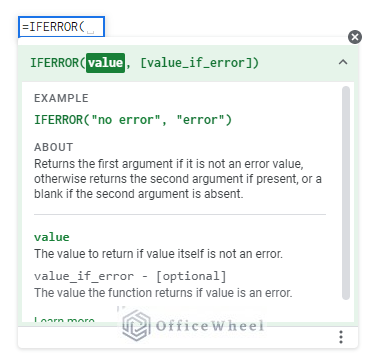
Arguments
The arguments of the IFERROR function are as follows:
| ARGUMENT | REQUIREMENT | FUNCTION |
|---|---|---|
| test_value | Required | The value that is being tested for error. It can be a cell reference or a formula. |
| value_if_error | Optional | The value that needs to be returned if the first parameter returns an error. |
Output
The formula =IFERROR(C5/D5, “N/A”) will look for an error; as an error is found, it returns the text ‘N/A’ as output.
3 Ideal Examples of Using the IFERROR Function in Google Sheets
As the Google Sheet IFERROR function deals with errors, it returns the first parameter if there is no error, otherwise if an error is found it returns the blank cell or specific instructed text. Here, we discuss some examples of using the IFERROR function in Google Sheets.
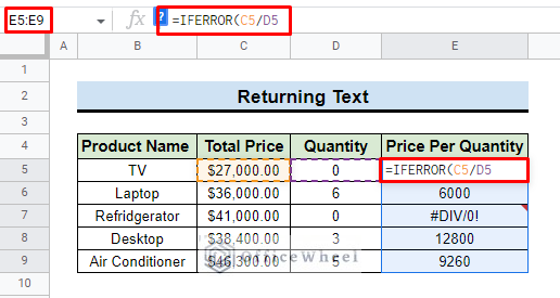
1. Return Values for General Errors
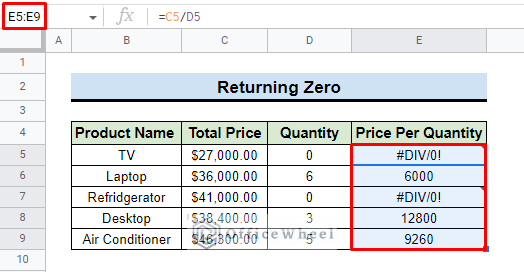
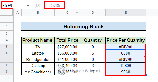
For applying the IFERROR function for general error, we develop a dataset that contains columns namely: Product Name, Total Price, Quantity, and Price Per Quantity.
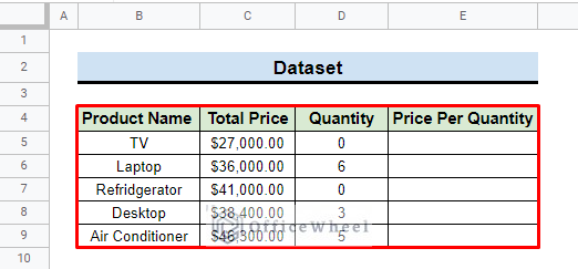
- To get the Price Per Quantity column we divided the total price by quantity and use the fill handle to apply the formula for the entire column.
- But #DIV/0! error was found, as some of the quantity values are 0.
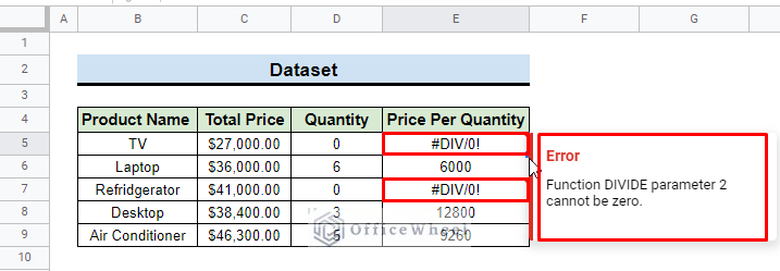
So, to clean up the dataset and transform the error message into a more systematic and logical approach. we will apply the following techniques:
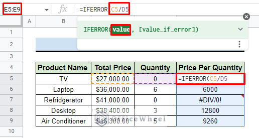
1.1 Return with Zero
If we want to replace the error with a zero(0) value,
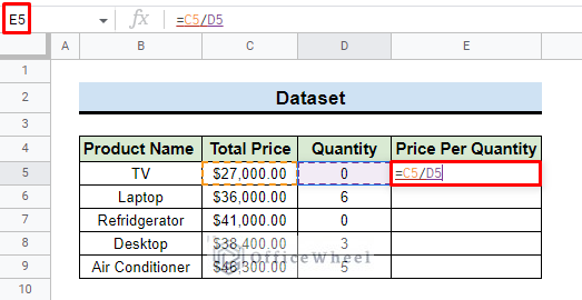
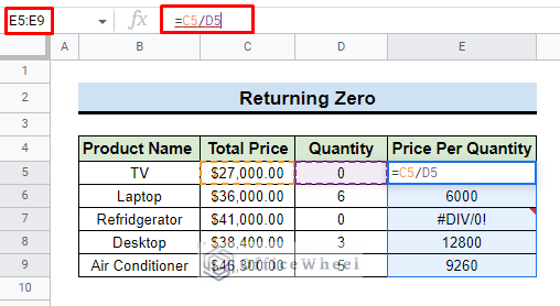
- First, Go and select the Price Per Quantity column where errors are found.
- Then go to the Formula bar and you will find the division formula.
- Now modify the formula by inserting the IFERROR function.
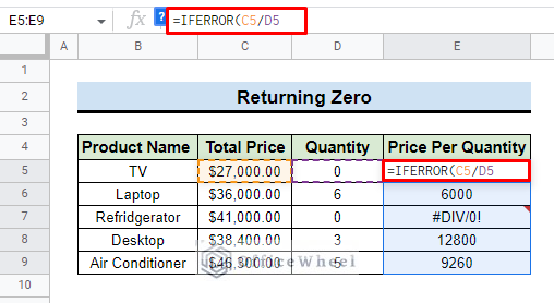
- The first argument keeps the same division formula that you applied before.
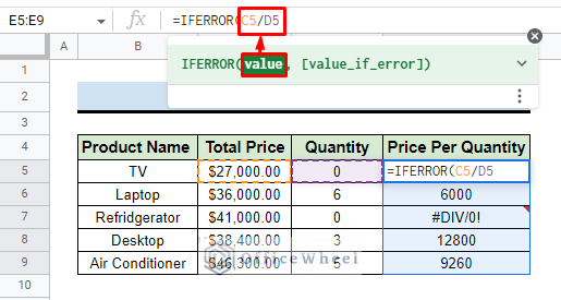
- After that for the value_if_error argument add “0” in the function.
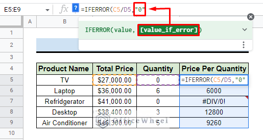
- Finally, press ENTER, and you will find a zero value in the place of the error.
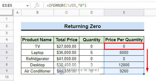
=IFERROR(C5/D5,”0”)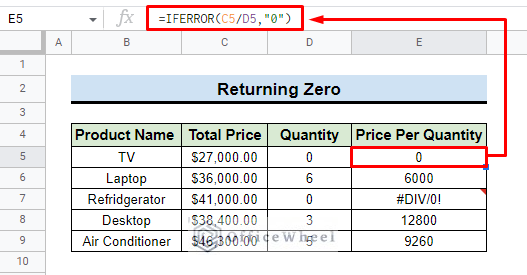
- You can use the Fill handle to insert the IFERROR function down the entire column.
Read More: [Fixed!] IFERROR Function Is Not Working in Google Sheets
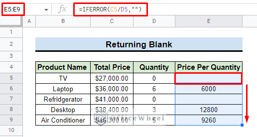
1.2 Return with Blank
If you want to keep the error cell blank,
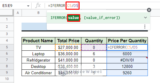
- Like the Return with Zero method, select the column and go to the Formula bar.
- Then insert the IFERROR function.
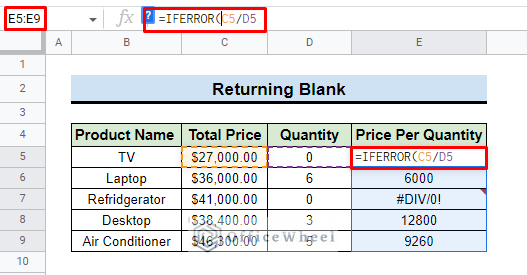
- Add the division formula as the value parameter of the function.
- After that for the value_if_error argument add “in the function.
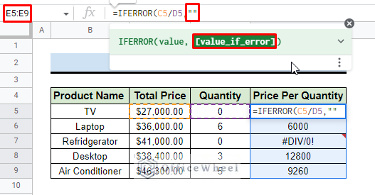
- Press ENTER and you will find a blank cell replacing the error value.
=IFERROR(C5/D5,””)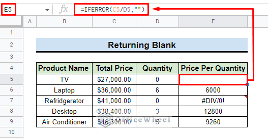
- At the end, use the Fill handle to apply the function to the entire column.
1.3 Return with Text
If you want to add any specific text, you have to go through the same process as we described before.
- Apply the IFERROR function for the Price Per Quantity column.
- Apply the existing division formula as the first parameter of the IFERROR function.
- Then add specific text “N/A” as the function’s second parameter.
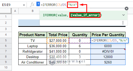
- Finally, press ENTER to apply the function and you will find the desired value in the selected cell.
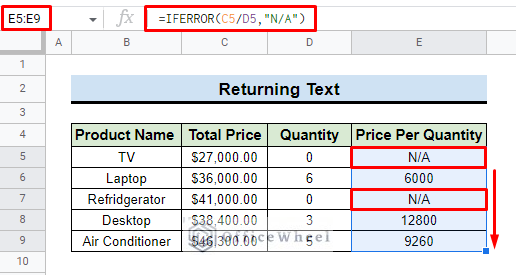
=IFERROR(C5/D5,"N/A")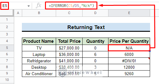
- Now apply the function to the entire cell by using the Fill Handle.
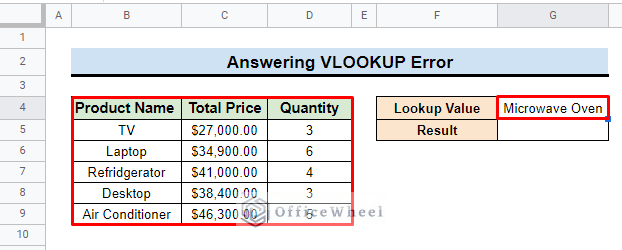
2. Answer with Specific Text During VLOOKUP Error
During applying the VLOOKUP function, When you look up a value that is unable to locate in the dataset, it returns a #N/A! error. Through the IFERROR function, you can replace the error with any meaningful text like ‘Not Found’, ‘Not in List’, or anything that supports the dataset.
Here, our dataset represents some product information and we look up a specific product “Microwave Oven”.
- Insert the VLOOKUP function in the G4 cell.
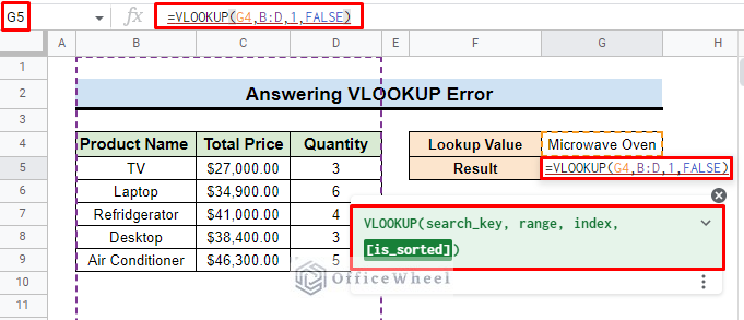
- Here, G3 is the search key, B:D represents the range, 1 is the column number from where to look up, and is_sorted set FALSE to get the exact value.
- Press ENTER and you will find a #N/A error in the result cell.
=VLOOKUP(G3,B:D,1,FALSE)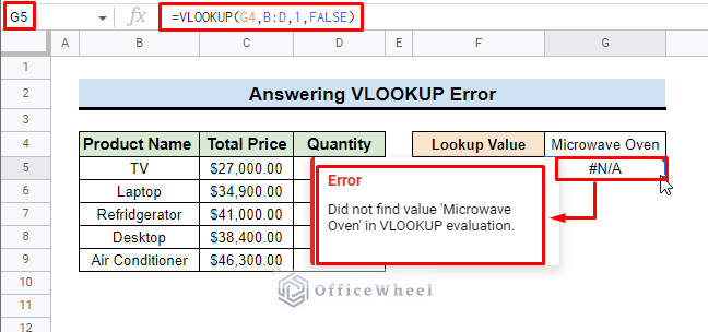
- To clear the error message and replace it with a meaningful message apply the IFERROR function before the VLOOKUP function in cell G5.
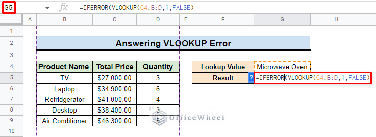
- The whole VLOOKUP function is considered the first argument.
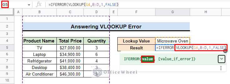
- After that, input “Not in List” as “value_if_error” in the function.
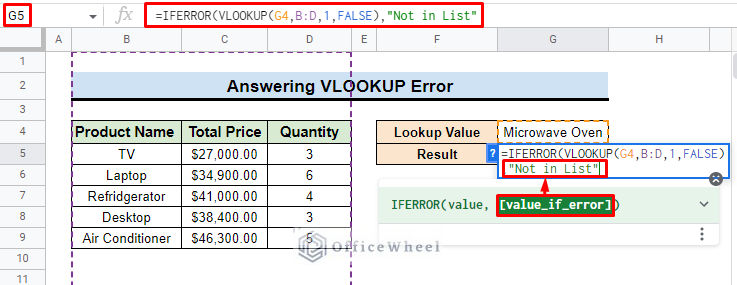
- Press ENTER and you will find your customized text in the selected cell.
=IFERROR(VLOOKUP(G4,B:D,1,FALSE),”Not in List”)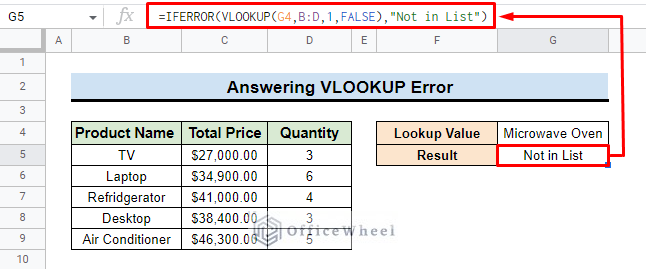
Read More: How to Use IFERROR with VLOOKUP Function in Google Sheets
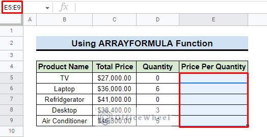
3. Use of IFERROR with ARRAYFORMULA Function
The ARRAYFORMULA function is used to calculate a range of data. You can apply the IFERROR function with the ARRAYFORMULA function to resolve error issues in your dataset. To do so,
- First, select the entire column where you want to insert the ARRAYFORMULA function. Here we select the Price Per Quantity column to apply the formula.
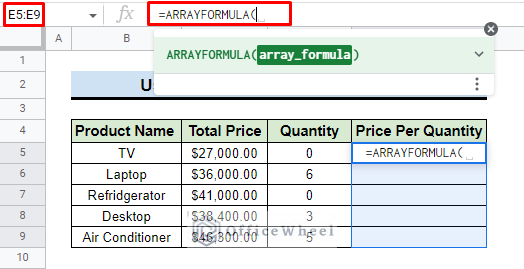
- Then go to the formula bar and insert the ARRAYFORMULA function.
- Now divide the C5:C9 range by the D5:D9 range.
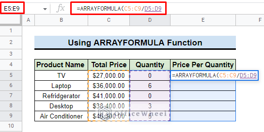
- Press ENTER and you will find the results with some errors in the entire column.
=ARRAYFORMULA(C5:C9/D5:D9)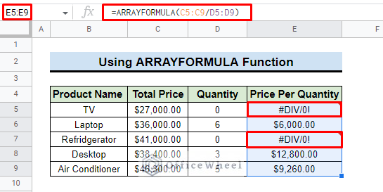
Note: Instead of typing the formula you can press CTRL+SHIFT+ENTER to apply ARRAYFORMULA.
- To resolve the error problem and remove the #DIV/0! Insert IFERROR function.
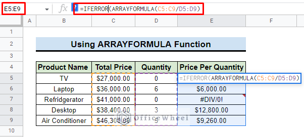
- The entire ARRAYFORMULA function considers the value parameter of the IFERROR function.
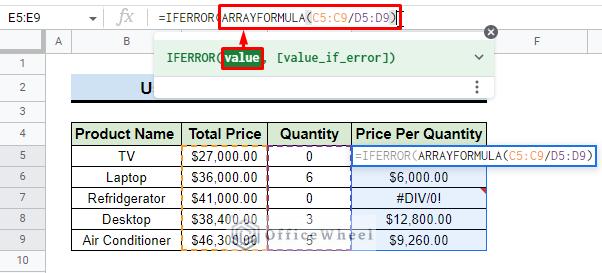
- Then insert the “” as value_if_error.
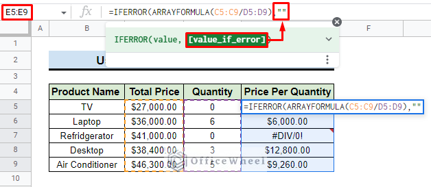
- Finally, press ENTER and you will find the error cells turn into the blank cell.
=IFERROR(ARRAYFORMULA(C5:C9/D5:D9),””)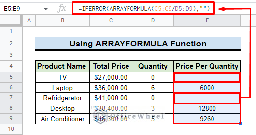
4. Other Types of Errors in Google Sheets
When you work in Google Sheets, you have to deal with different types of errors. But don’t worry. With the help of the IFERROR function, you can clean up all these from your dataset. Now, get to know about some of these errors and when they occur.
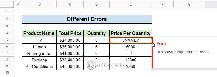
4.1 The #NAME? Error
This error generally occurs where there is a problem with the formula syntax. It may be a spelling mistake or a wrong name range.
Solution:
=IFERROR(C5/D5SG,"ERROR")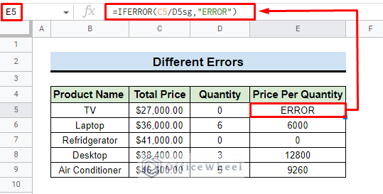
4.2 The #NUM! Error
This error returns when the Google Sheets has to display a large number value.
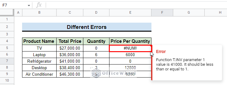
Solution:
=IFERROR(T.INV(C7,D7),"N/A")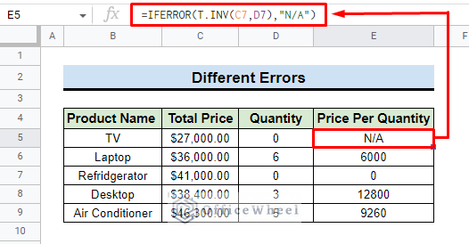
Conclusion
Hope this article helps you understand how to use IFERROR in Google Sheets and now you can easily hide or replace the error with a meaningful value. If you are keen to learn advanced functions in Google Sheets you can visit the OfficeWheel website.