The COUNTIF function is one of the most frequently used functions in Google Sheets. This function is helpful for counting the number of cells that meet a specific criterion. There are numerous instances for which we can use the COUNTIF function. In this article, I’ll discuss 7 simple examples of how to use the COUNTIF function in Google Sheets.
A Sample of Practice Spreadsheet
You can copy our practice spreadsheets by clicking on the following link. The spreadsheet contains an overview of the datasheet and an outline of the discussed examples of how to use the COUNTIF function in Google Sheets.
What Is COUNTIF Function in Google Sheets?
The COUNTIF function can return a count value depending on a specific condition.
Syntax
The syntax of the COUNTIF function is the following-
COUNTIF(range, criterion)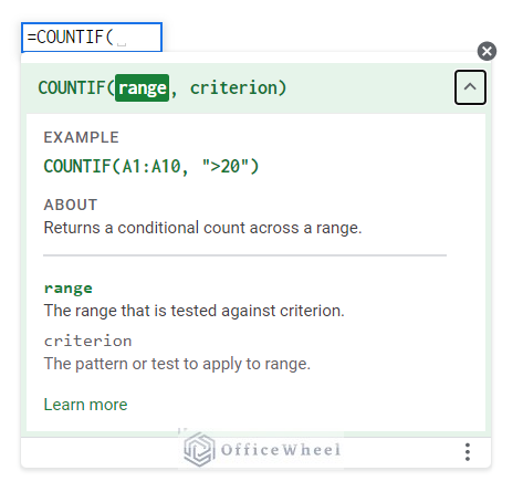
Argument
The arguments of the COUNTIF function are:
| Argument | Requirement | Function |
|---|---|---|
| range | Required | The range where criterion will be applied. |
| criterion | Required | The condition to be applied to the range for counting. |
Output
The formula =COUNTIF({1,27,6,7,12},”>3″) will return 4 as output.
7 Simple Examples to Use COUNTIF Function in Google Sheets
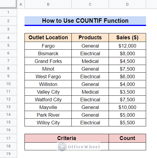
First, let’s get familiar with our dataset. The dataset contains a list of outlet locations, the type of products in that outlet, and the sales volume for that outlet. We’ll count cells from this dataset based on various criteria. Now let’s get started.
1. Applying for Comparison Operators
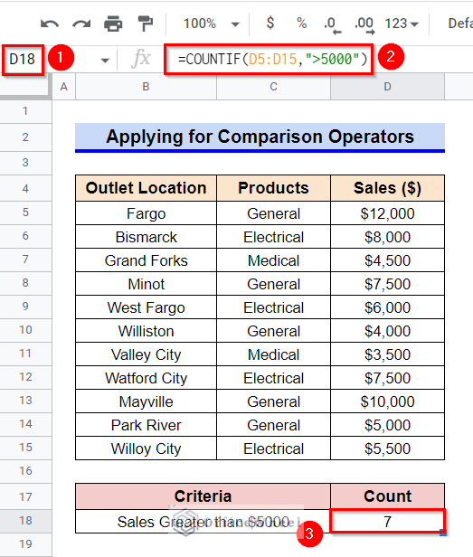
First, we will apply comparison operators in the criterion of the COUNTIF function. Various comparison operators like equal (=), less than (<), less than or equal (<=), greater than (>), greater than or equal (>=), and not equal(<>) can be used in Google Sheets. Here, we’ll use the greater than (>) comparison operator to calculate the number of cells that has a sales value higher than $5000.
Steps:
- Firstly, select Cell D18.
- Afterward, type in the following formula-
=COUNTIF(D5:D15,">5000")- Next, press the Enter key to get the required count.
Read More: How to Use COUNTIF for Cells Not Equal to Text in Google Sheets
2. Employing for Texts and Numbers Criterion
The text and number types of criteria are mostly used in Google Sheets. The COUNTIF function generally works only for an exact match with texts and number criteria.
2.1 Using with Text Criterion
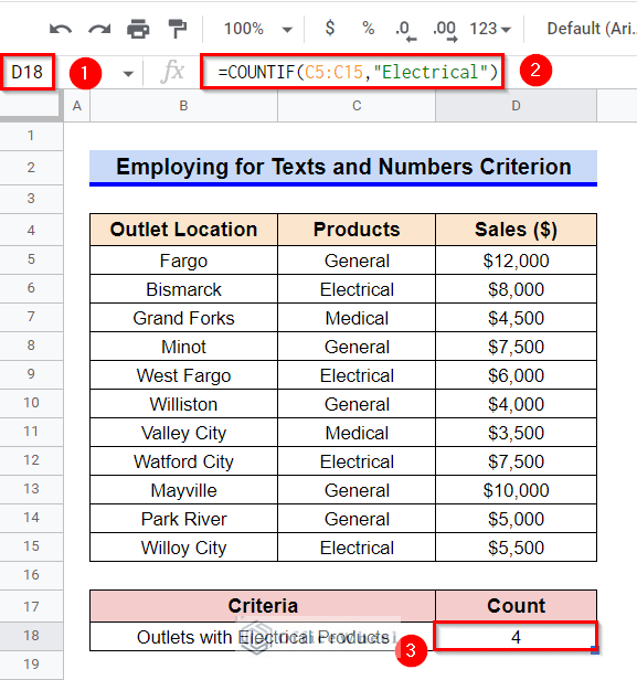
Here, we’ll compute the number of outlets with electrical products. One point to remember is that the text criterion we use in the COUNTIF function is not case-sensitive.
Steps:
- To start, activate Cell D18 by double-clicking on it.
- Next, type in the following formula-
=COUNTIF(C5:C15, "Electrical")- Concurrently, press Enter key to get the required output.
Read More: How to Execute Case Sensitive COUNTIF in Google Sheets
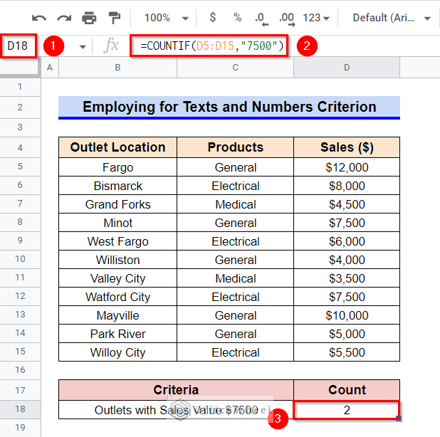
2.2 Implementing for Number Criterion
Implementing a number criterion is very similar to the process of applying a text criterion. Here, we’ll calculate the number of outlets with a sales value equal to $7500.
Steps:
- Select Cell D18 first and then, type in the following formula-
=COUNTIF(D5:D15, "7500")- After that, get your required count by pressing the Enter button.
Read More: COUNTIF Function with “Not Equal to” Criterion in Google Sheets
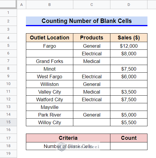
3. Counting Number of Blank Cells
A blank cell is often used in our datasets if we don’t have appropriate data for that cell. So, we may require to calculate the total number of blank cells in a dataset. Here, we have left a few blank cells to demonstrate this and the next example.
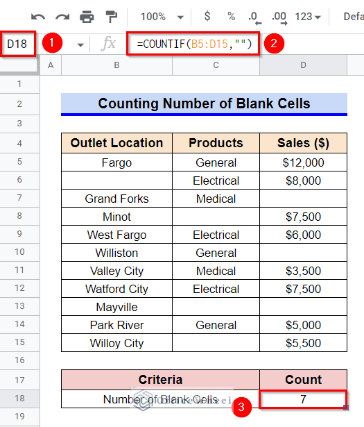
Steps:
- Activate Cell D18 by selecting it first and then using the function key F2.
- Afterward, type in the following formula-
=COUNTIF(B5:D15,"")- Finally, press the Enter key to get the required result.
Read More: Google Sheets Count Cells from Another Workbook with COUNTIF Function
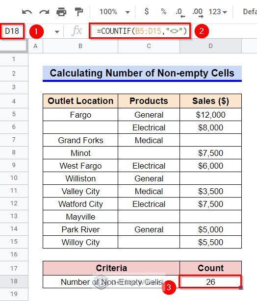
4. Calculating Number of Non-empty Cells
We can also calculate the number of non-empty cells in a data range. The formula is very similar to the previous examples, we just require a criterion that depicts the non-empty cells. Now let’s get started.
Steps:
- To start, activate Cell D18 by double-clicking on it.
- Now, insert the following formula-
=COUNTIF(B5:D15,"<>")- Consequently, get your required result by pressing the Enter key.
Read More: [Fixed!] COUNTIF Function Is Not Working in Google Sheets
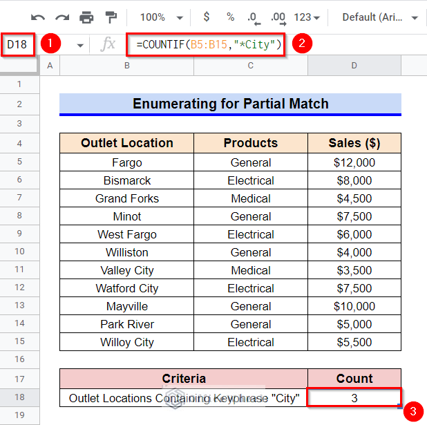
5. Enumerating for Partial Match
Although the COUNTIF function generally enumerates for exact matches, we can also apply it for partial matches by using wildcard characters. Three wildcard characters are used in Google Sheets. They are the asterisk (*), which is used for finding a number of characters, the question mark (?), which is used for finding a single character and the tilde (~), used before “*” or “?” if these characters are not used as wildcard characters.
5.1 Using Asterisk Wildcard Character
Let’s find the number of outlet locations that contain the keyphrase “City” in their name. Since we are looking for a number of characters, we’ll use the asterisk (*) symbol here.
Steps:
- First, activate Cell D18 by double-clicking on it.
- Afterward, type in the following formula-
=COUNTIF(B5:B18, "*City")- Finally, get the required count of the partial match by pressing the Enter button.
Read More: Use COUNTIF If Cell Contains Specific Text in Google Sheets
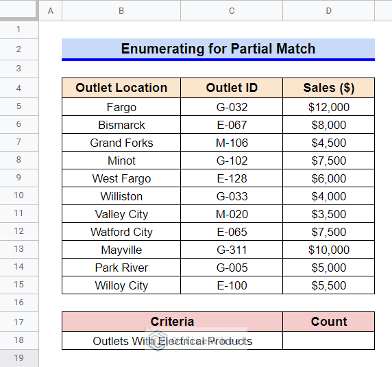
5.2 Using Question Mark Wildcard Character
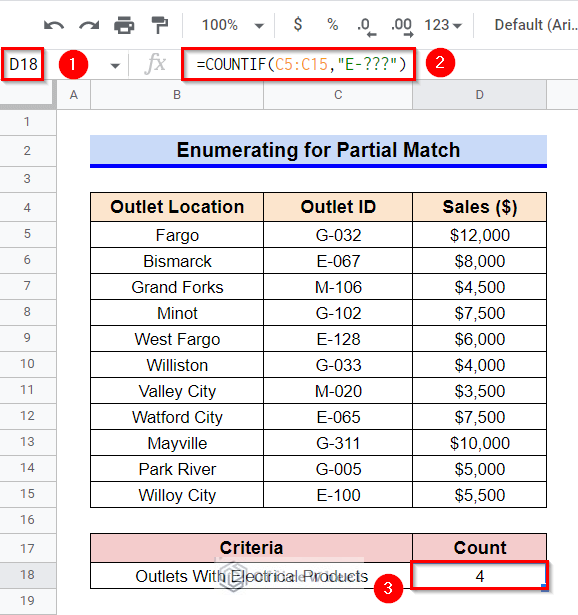
Here, we have modified our dataset a little to demonstrate an example with the question mark (?) wildcard. The product types of an outlet will be understood by a unique Outlet ID which is basically a 5-digit code. The first digit represents the product types in that outlet. We’ll compute the number of outlets with electrical products. The initial two digits are E- for such outlets.
Steps:
- Activate Cell D18 by selecting it first and then using the function key F2.
- After this, insert the following formula-
=COUNTIF(C5:C15,"E-???")- The three question marks refer to three random digits after the two initial specified digits.
- Finally, press the Enter key to get the required output.
Read More: How to Use VLOOKUP with COUNTIF Function in Google Sheets
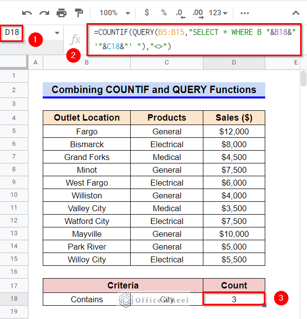
6. Combining COUNTIF and QUERY Functions
We can use the QUERY function to get a range for the COUNTIF function instead of using wildcard characters in the criterion. In fact, employing the QUERY function can help the COUNTIF function to be executed for a wider set of instances. Here, we’ll compute the number of cells that contain the keyphrase “City”.
Steps:
- Firstly, select Cell D18.
- Afterward, type in the following formula-
=COUNTIF(QUERY(B5:B15,"SELECT * WHERE B "&B18&" '"&C18&"' "),"<>")- Finally, get the required output by pressing the Enter button.
Formula Breakdown
- QUERY(B5:B15,”SELECT * WHERE B “&B18&” ‘”&C18&”‘ “)
First, the QUERY function runs a Google Visualization API Query Language query across the range B5:B15. The expression SELECT * WHERE starts a query. Next expression B indicates the query run in Column B. And the expression “&B18&” indicates the query operator. The & symbols are used for extracting the text from Cell B18. The expression ‘“&C18&”’ indicates the cell reference of the search term. The apostrophes (‘’) symbol differentiates the search term from the search operator.
- COUNTIF(QUERY(B5:B15,”SELECT * WHERE B “&B18&” ‘”&C18&”‘ “),”<>”)
Next, the COUNTIF function counts the number of non-empty cells returned by the QUERY function.
7. Using COUNTIF Function for Multiple Criteria
Although the COUNTIF function can deal with only one criterion, we can add or subtract multiple COUNTIF functions to execute multiple criteria. Keep reading to learn how.
7.1 Applying COUNTIF Function for OR Logic
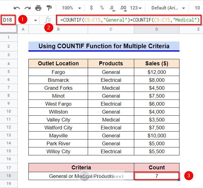
To execute a logical OR criterion in the COUNTIF function, we have to add multiple COUNTIF functions. Here, we’ll calculate the number of outlets with General or Medical products.
Steps:
- First, activate Cell D18 by double-clicking on it.
- Then, insert the following formula-
=COUNTIF(C5:C15,"General")+COUNTIF(C5:C15,"Medical")- Consequently, get the required output by pressing Enter button.
Formula Breakdown
- COUNTIF(C5:C15,”General”)+COUNTIF(C5:C15,”Medical”)
The first COUNTIF function returns the number of outlets with the general type of products. Similarly, the second COUNTIF function returns the number of outlets with medical products. Later, they are added to calculate the count of outlets with general or medical products.
7.2 Employing COUNTIF Function for AND Logic
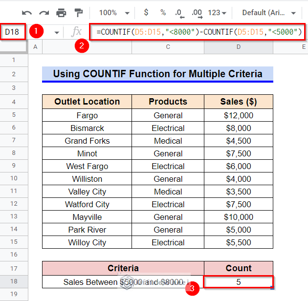
The execution of a logical AND criterion is similar to the execution of a logical OR criterion. Except, we need to subtract the COUNTIF functions this time. However, we can apply the COUNTIFS function instead in these instances. Now, let’s calculate the number of outlets with sales value between $5000 and $8000.
Steps:
- Firstly, select Cell D18 and then type in the following formula-
=COUNTIF(D5:D15,"<8000")-COUNTIF(D5:D15,"<5000")- Now, press the Enter key to get the required output.
Formula Breakdown
- COUNTIF(D5:D15,”<8000″)-COUNTIF(D5:D15,”<5000″)
The first COUNTIF function returns the number of outlets with a sales value lower than $8000. Similarly, the second COUNTIF function returns the number of outlets with a sales value lower than $5000. Later, they are subtracted to calculate the count of outlets with sales between $5000 and $8000.
How to Apply COUNTIF Function with Conditional Formatting in Google Sheets
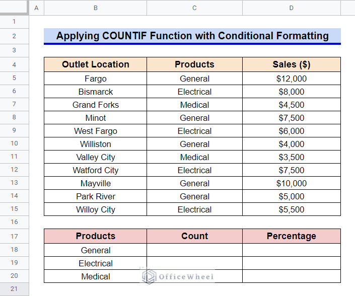
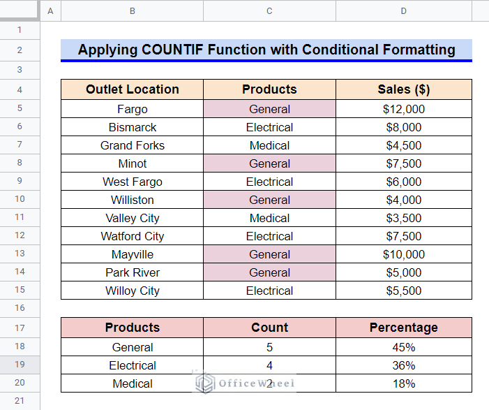
We can also apply COUNTIF functions to format a data range based on a specific condition. Here, we’ll highlight the outlets with similar product types using a particular color. We need to modify our dataset like the following for that. We also require the SUM function for this example.
Steps:
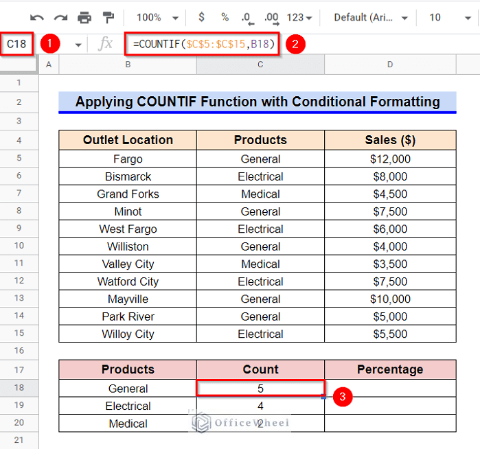
- First, we have to count the number of outlets based on the type of product.
- Calculated the number of outlets with general types of products in Cell C18, using the following formula-
=COUNTIF($C$5:$C$15,B18)- Later, use the Fill Handle icon to copy the formula to the other two cells.
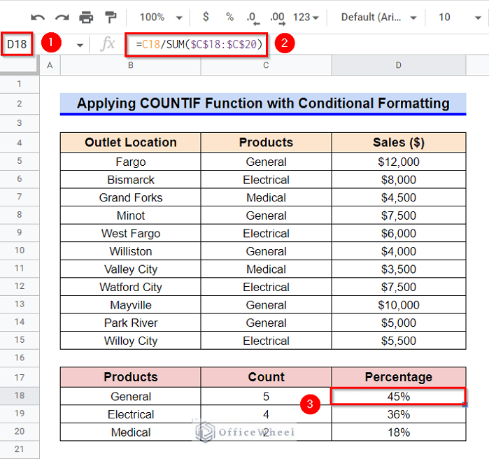
- Now, let’s calculate the percentage of outlets based on product types.
- Insert the following formula in Cell D18 and then press Enter key for this.
=C18/SUM($C$18:$C$20)- Format the value as a percentage and then copy it to the other two cells by using the Fill Handle tool.
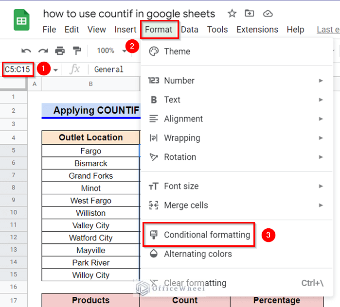
- At this point, select the range C5:C18 and go to the Format menu.
- Then, select Conditional Formatting from the appeared options.
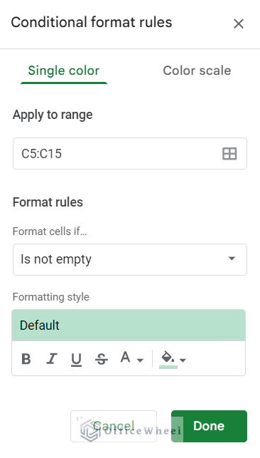
- A sidebar like the following will appear.
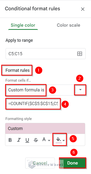
- Here, set the Format Rules to Custom Formula from the dropdown list.
- Afterward, set the formula to the following-
=COUNTIF($C$5:$C$15,C5)/COUNTIF($C$5:$C$15,"*")>0.4- Consequently, select the required fill color from Formatting Style.
- And now, click on Done.
Formula Breakdown
- COUNTIF($C$5:$C$15,C5)/COUNTIF($C$5:$C$15,”*”)>0.4
The percentage of outlets with General types of products is 45%. Hence, we have used two COUNTIF functions to check for which cells the proportion is greater than 0.4 and apply conditional formatting to those cells. The first COUNTIF function returns the number of cells in the range C5:C15 that match the content of Cell C5. And the second COUNTIF function returns the number of non-empty cells in the range C5:C15.
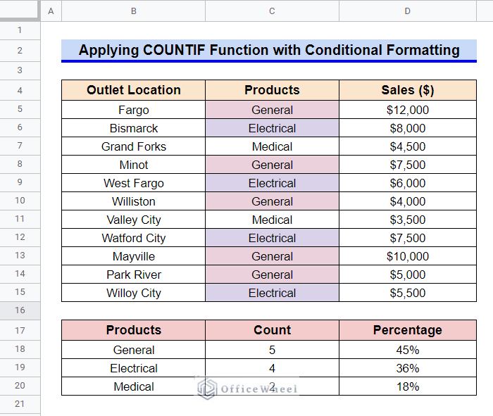
- The dataset now looks like the following.
- Now, similarly, add another conditional format like the following image.
- Use the following formula in the Custom Formula of Format Rules.
=COUNTIF($C$5:$C$15,C5)/COUNTIF($C$5:$C$15,"*")>0.3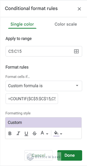
- As soon as we click on Done in the sidebar, the dataset will look like the following. As you can see the cells with different types of products are formatted differently.
Read More: COUNTIF with Greater than and Less than Criteria in Google Sheets
Things to Be Considered
- Unless you are using a cell reference, you have to insert the criterion in a set of double quotation marks (“”).
Conclusion
This concludes our article to learn how to use the COUNTIF function in Google Sheets. I hope the demonstrated examples were ideal for your requirements. Feel free to leave your thoughts on the article in the comment box. Visit our website OfficeWheel.com for more helpful articles.