When working with a large volume of data, we may need to check if a value exists within a specified range. This can be time-consuming and have the potential of being error-prone. In such cases, Google Sheets provides some easy ways with which we can check if a value exists in range in Google Sheets.
A Sample of Practice Spreadsheet
Download this spreadsheet to practice yourself.
4 Simple Methods to Check If Value Exists in Range in Google Sheets
In this article, we will discuss 4 easy methods to check if a value exists in a range of cells in Google Sheets.
Method 1: Using COUNTIF Function
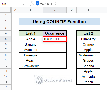
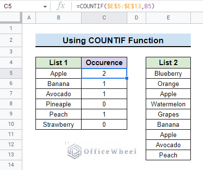
The COUNTIF function can be used to count the occurrences of a specific value in a range. We use the following dataset which has two lists with fruit names. We will see whether or not fruit from List 1 exists in List 2 using the COUNTIF function.
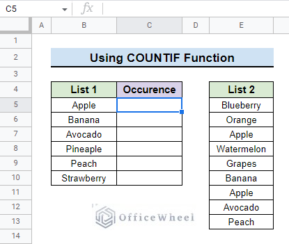
- At first, go to the cell where you want to show the count. We go to cell C5 in our example.
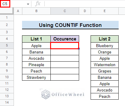
- Then, insert the COUNTIF function.
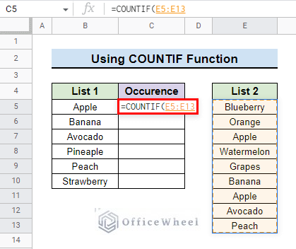
- After that, insert the range where you want to look up the value. We type E5:E13 in our example.
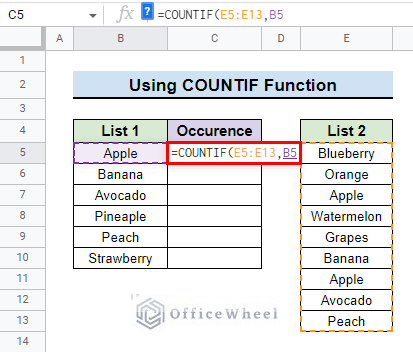
- Then, type the criterion of the COUNTIF function that is the value you want to look up in the range. We type B5.
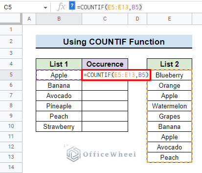
- This is what the final formula looks like:
=COUNTIF($E$5:$E$13,B5)- Finally, press ENTER to show the occurrence of value. If a value does not exist within the range, the formula will return 0. If it exists one time then the formula will return 1 and so on.
Method 2: Applying IF Function with COUNTIF Function
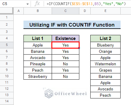
The COUNTIF function cannot show a specific message if a value exists within a range. It only shows the number of occurrences. We can use the IF function with the COUNTIF function to show a specific message if a value exists in a range.
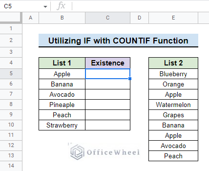
The dataset that we used for this method is the same as the previous method. We will show if fruit from List 1 exists in List 2 and show a Yes message if it exists and a No message if it does not exist using the IF function and the COUNTIF function.
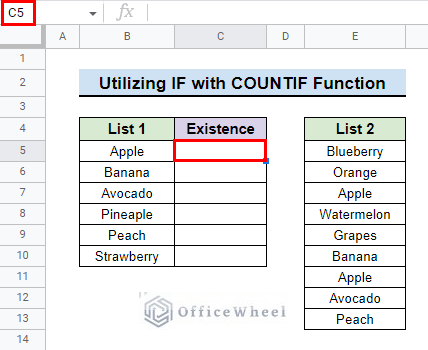
- At first, go to the cell where you want to show the message. We go to cell C5.
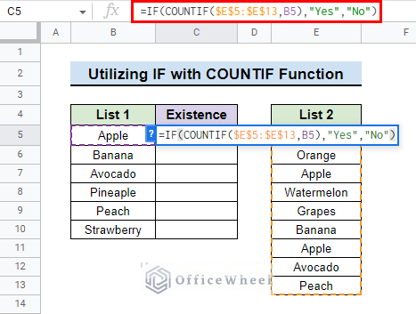
- Then, type the following formula:
=IF(COUNTIF($E$5:$E$13,B5),"Yes","No")Formula Explanation:
- COUNTIF($E$5:$E$13,B5)
First, the COUNTIF function returns the occurrences of the values in the range E5:E13.
- IF(COUNTIF($E$5:$E$13,B5),”Yes”,”No”)
Then, the IF function will show the Yes message if the value exists in the range E5:E13 otherwise, it will show the No message.
- Finally, press ENTER to show a message if the fruit name from List 1 exists in List 2.
Read More: Highlight Cell If Value Exists in Another Column in Google Sheets
Similar Readings
- VLOOKUP Error in Google Sheets (with Quick Solutions)
- Combine VLOOKUP and HLOOKUP Functions in Google Sheets
- Create Hyperlink to VLOOKUP Cell in Multiple Rows in Google Sheets
- Alternative to Use VLOOKUP Function in Google Sheets
- How to Use VLOOKUP for Conditional Formatting in Google Sheets
Method 3: Utilizing MATCH Function with IF and ISERROR Functions
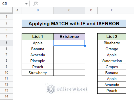
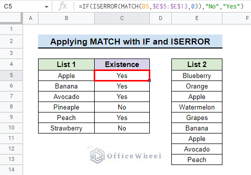
The MATCH function can be used with the IF and the ISERROR function to show if a value exists in a range. For this method, we use the same dataset that we used for the previous methods. We will show if fruit from List 1 exists in List 2 and show a Yes message if it exists and a No message if it does not exist using the IF and the ISERROR function in combination with the MATCH function.
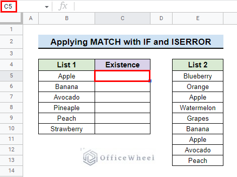
- At first, go to the cell where you want to show the result. We go to cell C5 in our example.
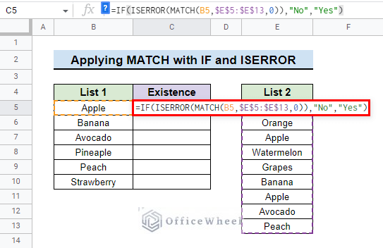
- Then, type the following formula:
=IF(ISERROR(MATCH(B5,$E$5:$E$13,0)),"No","Yes")Formula Explanation:
- MATCH(B5,$E$5:$E$13,0)
First, the MATCH function will find the value in the range E5:E13 and will show the row number of the table where it exists.
- ISERROR(MATCH(B5,$E$5:$E$13,0))
Then, the ISERROR function will return a FALSE message if the MATCH function can find the value in the range E5:E13 otherwise, it will return a TRUE message.
- IF(ISERROR(MATCH(B5,$E$5:$E$13,0)),”No”,”Yes”)
Finally, the IF function will return a No message when the ISERROR function returns a TRUE message and it will return a Yes message when the ISERROR returns a FALSE message.
- Finally, press ENTER to show the result. The formula will return a Yes message if the value from List 1 exists in List 2 and a No message if the value does not exist in List 2.
Read More: How to VLOOKUP All Matches in Google Sheets (2 Approaches)
Method 4: Checking with VLOOKUP, IF, and IFERROR Functions
The VLOOKUP function can be used with the IF function and the IFERROR function to show if a value exists in a range. It can be done only for numerical values. The previous three methods can be used both for numerical and text values.
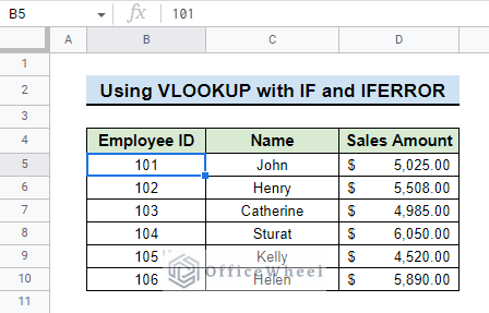
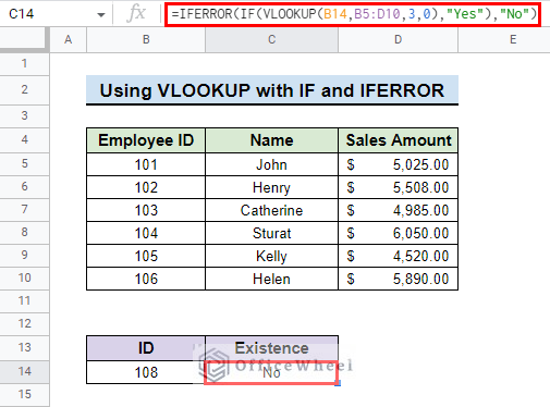
Consider the following dataset with Employee Id, Name, and their respective Sales Amount. We will show if an Employee Id exists in the table by using a formula using VLOOKUP, IF, and IFERROR functions.
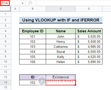
- At first, go to the cell where you want to show the result. We go to cell C14 in our example.
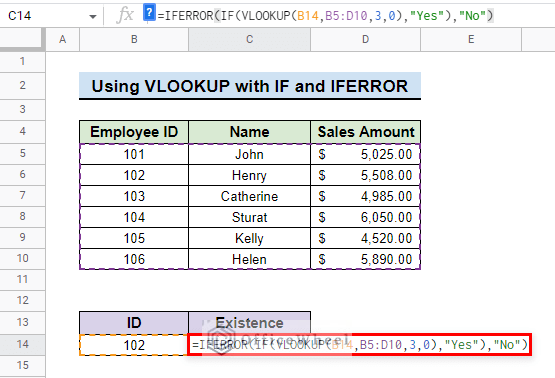
- Then, insert the following formula:
=IFERROR(IF(VLOOKUP(B14,B5:D10,3,0),"Yes"),"No")Formula Explanation:
- VLOOKUP(B14,B5:D10,3,0)
First, the VLOOKUP function will look for the value in the range B5:D10 and will return a value from the 3rd column of the same range if it can find a match.
- IF(VLOOKUP(B14,B5:D10,3,0),”Yes”)
Then, the IF function will return a Yes message if the VLOOKUP finds a match otherwise, it will return a #N/A error message.
- IFERROR(IF(VLOOKUP(B14,B5:D10,3,0),”Yes”),”No”)
Finally, the IFERROR function will return a No message when the IF function returns a #N/A error implying that the value does not exist in range B5:D10.
- Finally, press ENTER to show if the value exists in a range. We can see that the formula returns a Yes message as the value exists in the range.
- The formula will return a No message if the value does not exist in the range.
Read More: How to Use IFERROR with VLOOKUP Function in Google Sheets
Conclusion
In this article, we showed you 4 methods to check if a value exists in the range in Google Sheets. Keep practicing the methods that we have shown here for a better understanding of the concept. We hope this article was useful to you to help you.
Also, check out other articles on OfficeWheel to keep on improving your Google Sheets work knowledge.
Related Articles
- Google Sheets Vlookup Dynamic Range
- How to Use VLOOKUP with Named Range in Google Sheets
- How to Use Wildcard in Google Sheets (3 Practical Examples)
- How to Use Nested VLOOKUP in Google Sheets
- [Fixed!] Google Sheets If VLOOKUP Not Found (3 Suitable Solutions)
- How to Use VLOOKUP Function for Exact Match in Google Sheets
- How to VLOOKUP Multiple Columns in Google Sheets (3 Ways)
- How to Use VLOOKUP with Drop Down List in Google Sheets

