Google Sheets: How to Autofill Based on Another Field (4 Easy Ways)

The term Autofill can take many forms in Google Sheets, of which the most common is the fill-down columns method in a worksheet. On the other hand, we can also autofill cells based on the values in another cell, field, or even a different worksheet in Google Sheets.

These types of auto-fills are highly conditional and mostly implemented using functions or formulas.

Let’s see how we can do that in this article.

4 Ways to Autofill Based on Another Field in Google Sheets

1. Using the IF Statement to Autofill Cells Based on Text in Another Field

The simplest way to implement conditions in a spreadsheet is by using an IF statement. In other words, the IF function.

The IF function syntax:

For example, let’s say we want to autofill the Result column based on the values of the Score column in the following worksheet:

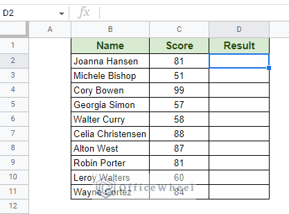
Step 1: Enter the following IF formula in the first cell of the Result column:

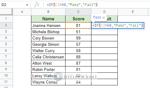
The formula checks the value of the adjacent cell of the Score column. Depending on the field value, the formula presents a result of either “Pass” or “Fail”.

Step 2: Use the fill handle to autofill the formula down the column of Google Sheets. This will automatically generate the results in the column.

For Multiple Conditions

We also can apply the IF statement for multiple conditions using the IFS function.

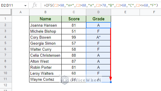
To use an example, let’s say we want to specify the Grades according to the Scores achieved by each student.

Step 1: Apply the IFS formula with each individual condition for the grade:

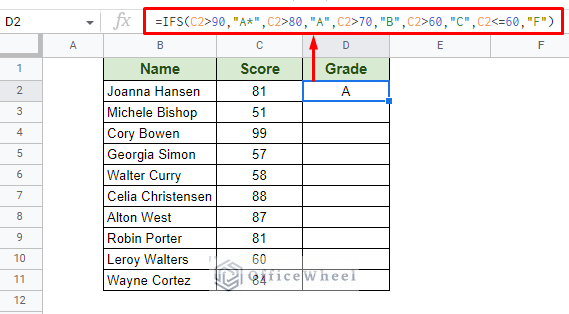
Step 2: Use the fill handle to autofill the formula to the rest of the column.

2. Using VLOOKUP to Autofill Based on Another Field in Google Sheets

Another way to approach autofill is to extract a value depending on the value of another field. For this particular condition, we have the VLOOKUP function.

The VLOOKUP function syntax:

Consider the following worksheet for example:

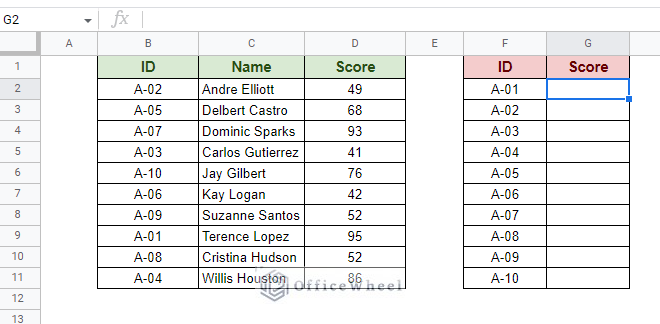
Here, we want to extract the scores of the respective ID numbers in the second table.

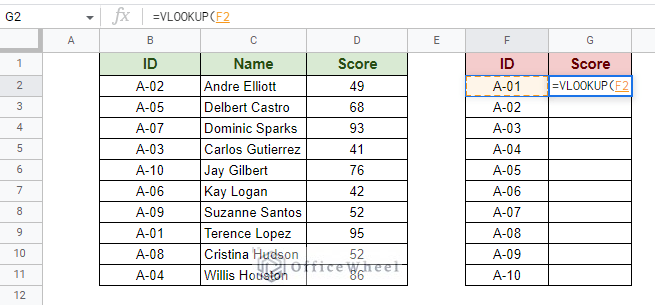
Step 1: Open the VLOOKUP function in the cell. Enter the search key, which in this case is in cell F2.

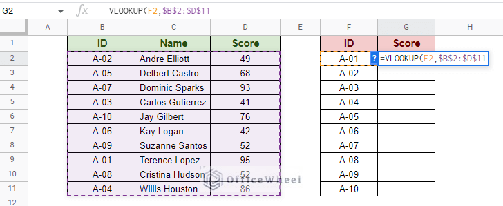
Step 2: Input the data range. The range of the first table.

Step 3: Input the column index to extract the desired value. Since Score is the third column of our data range, the column index will be 3.

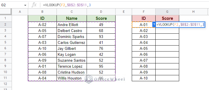
Step 4: We’ll leave the [is_sorted] field as FALSE. Close parentheses and press ENTER to autofill the column based on the Scores obtained by the left field ID in Google Sheets.

Use the fill handle to auto-fill the rest of the column.

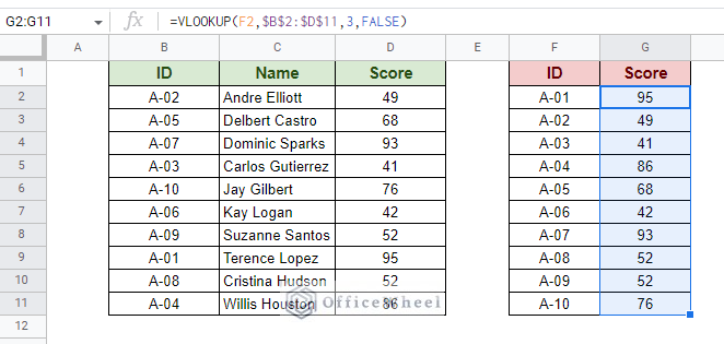
Note: Leaving the data range reference locked with absolutes ($) is recommended.

VLOOKUP From Another Worksheet And Autofill Based on the Values There

The source dataset or table does not have to be in the same worksheet. The VLOOKUP function is versatile enough to be able to extract data from different worksheets in Google Sheets.

Consider our previous example, only this time the source data is in a separate worksheet.

To bring in data from another worksheet, we only need to change the cell reference:

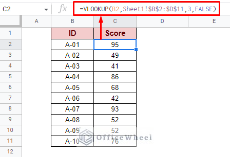
Whichever method you follow, the results will remain dynamic as long as it is within the range.

3. Autofill Columns to the Right Based on Values in the Left in Google Sheets (Quick Data Entry of Existing Values)

We all know that data entry can be a tedious task. A boring repetition of the same value inputs.

What if we said we can automate the process with nothing more than a simple formula?

What we mean is this:

It is possible to autofill columns based on the value of another cell in Google Sheets using virtually nothing but a VLOOKUP formula.

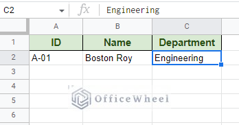
Step 1: Input the first data entry. This is important as the formula requires a starting point.

Step 2: Apply the following formula in the second/adjacent column, which in our case is cell B3.

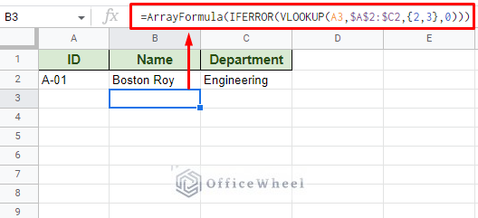
The formula requires a left-side value to base the autofill from.

Since we want to autofill the Name and Department fields, we must input two indexes: 2 and 3. This is inputted as an array, thus the curly braces {}. This is also the reason why we include ARRAYFORMULA.

IFERROR returns a blank cell if the adjacent cell in the ID column is blank.

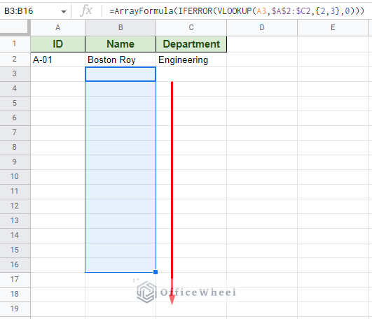
Step 3: Apply the formula to the rest of the column (you set the limit) with the fill handle.

Note: If you have more than two columns you want to autofill, simply include the column indexes within the curly braces, e.g. {2, 3, 4, 5, … n}. Non-adjacent column indexes will also work.

At this point, if an ID is repeated, the left adjacent columns will autofill based on the input ID.

If a new ID is inputted here, there will be no autofill. You can simply overwrite the formula with a value without affecting the rest of the column.

The method in action:

4. Using FILTER Function to Autofill Based on Another Field

The FILTER function is another great way to autofill data based on the value of another field in Google Sheets.

The FILTER function syntax:

Consider the following worksheet:

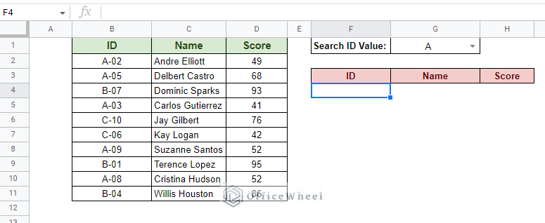
What we look to do here is to generate or autofill the values of the source data based on the value given by the “Search ID Value” field of this Google Sheets worksheet.

We use this FILTER formula:

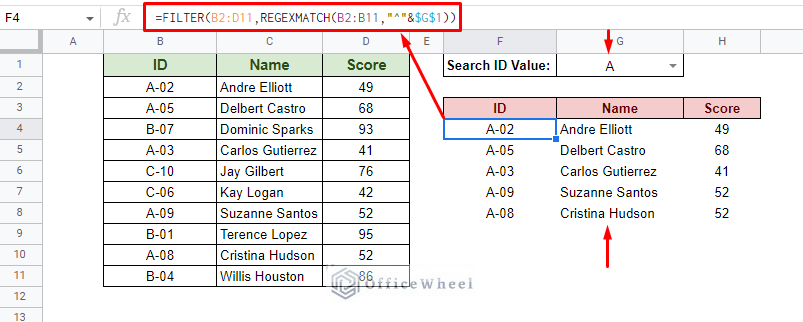
The FILTER function is quite dynamic as it automatically presents all matched values in an array without the use of ARRAYFORMULA. And with referencing the match criteria, we can go a step further with the dynamism.

Learn More: Google Sheets: Filter Data if it Contains Value (A Comprehensive Guide)

Final Words

As we have seen in this article, any function that can take conditions may be utilized to autofill data according to their respective functionalities. Of which, the VLOOKUP function seems the most versatile when we want to autofill based on another field in Google Sheets.

Feel free to leave any queries or advice you might have for us in the comments section below.

Related Articles

• How to Autofill Formula in Google Sheets (3 Easy Ways)
• How to Autofill Numbers in Google Sheets (An Easy Guide)