In this simple tutorial, we will show you how you can find all cells with value in Google Sheets. Be it any value or specific value (text or otherwise) that you are looking for.
Let’s get started.
3 Ways to Find All Cells With Value in Google Sheets
1. Find Cells With Specific Value in Google Sheets
To search for any specific value in Google Sheets, whether it be a number or text, we first look toward the LOOKUP functions.
I. LOOKUP Function
The base LOOKUP function works with only sorted data from one range. It can find a value within the range and return a value corresponding to it.
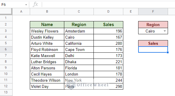
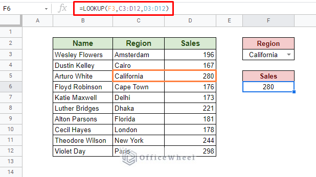
For example, we have the following worksheet of employee Names, their Region, and the number of Sales they have achieved. We will look to search and retrieve the Sales numbers according to the region.
Our formula:
=LOOKUP(F3,C3:D12,D3:D12)Formula Breakdown:
- The specific value that we are searching for is the Sales number for the region California, making California our search_key, cell F3.
- Our range of values is C3:D12. The function will look for both the search_key and result from within this range. If not found, we will get an error.
- D3:D12 is our result_range. The value that is extracted corresponds to the row that our search value is in.
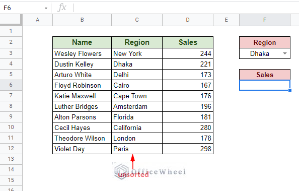
Note that in most cases, the dataset will not be sorted as we have seen just now. For unsorted data, and frankly, for a better method for finding cells with value, we resort to the VLOOKUP function.
Read More: How to Find the Range in Google Sheets (with Quick Steps)
II. VLOOKUP Function
We now have the following dataset where the columns are not sorted:
The VLOOKUP function’s advantage comes from the ability to work with unsorted data correctly. This makes the function the best method to search and find specific values in a range in Google Sheets.
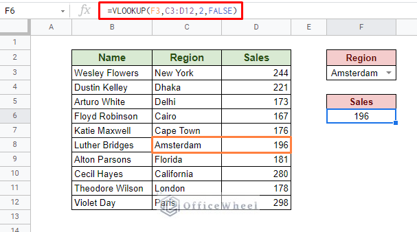
Our example is the same as before: Return the Sales number for a specific region.
=VLOOKUP(F3,C3:D12,2,FALSE)Formula Breakdown:
- Same as LOOKUP, our search_key is in cell F3.
- C3:D12 is our data range. It should include the search key and result columns. If the search value is not found, we will get an error.
- The 2 is the index number of our data range. This represents the column number from which the result is extracted corresponding to the search key.
- Since our dataset is not sorted, the [is_sorted] field is FALSE. This helps us get the exact match in the range.
While VLOOKUP may be a great function to find specific values in a range in Google Sheets, it is not perfect.
Limitations of VLOOKUP
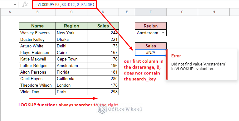
- The search_key must be in the first column of the selected data range. Otherwise, the function will not find it.
- All LOOKUP functions look toward the right, as defined by the index number. We cannot lookup values to the left, for example, the Name column in our dataset.
To learn more about finding values in a range, please see our Find Value in a Range in Google Sheets article.
III. Using the INDEX-MATCH Combination
The INDEX MATCH function combination remedies any limitations that we have seen in the VLOOKUP function. With this formula, we can define any column to have our search value and result, regardless of their position.
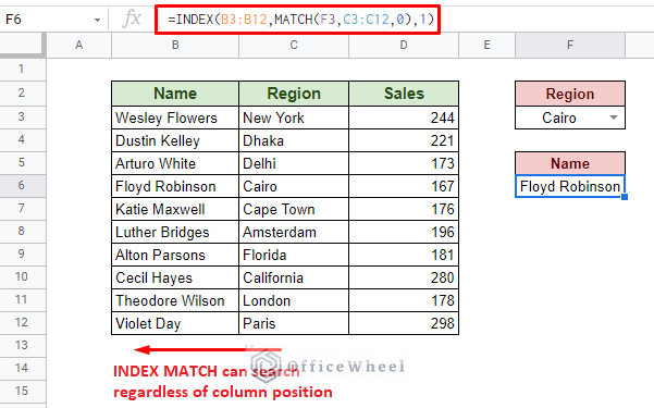
For example, let’s say we want to find the Name of the employee corresponding to the Region. Our formula:
=INDEX(B3:B12,MATCH(F3,C3:C12,0),1)The result column is defined by the reference field of the INDEX function. The search key for the specific value is covered by the MATCH function (taking reference from F3 and the Region column).
Read more: Use of Google Sheets INDEX MATCH in Multiple Columns
IV. Only Find All Cells Containing Value
Coming away from what we have just discussed, if you are looking for a way to only find the cells that contain a specific value, you need not look further than the Find and Replace option of Google Sheets.
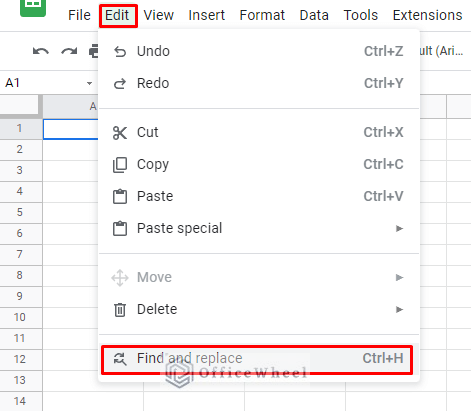
You can access the option from the Edit tab. Keyboard shortcut: CTRL+H
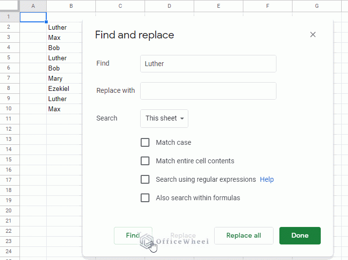
Simply input your search text and click Find to highlight the cell. Keep on clicking Find to cycle through all occurrences.
While this method does not list the values or occurrences within the spreadsheet, it has other significant search uses.
Alternatively, CTRL+F also works just fine.
Read More: Find and Replace in Google Sheets
Similar Readings
- How to Find Hidden Rows in Google Sheets (2 Simple Ways)
- Find Cell Reference in Google Sheets (2 Ways)
- How to Use FIND Function in Google Sheets (5 Useful Examples)
- Use REGEXREPLACE to Replace Multiple Values in Google Sheets (An Easy Guide)
2. Find All Cells with Any Value in Google Sheets (Non-Empty Cells)
Our focus for this section is to find all cells containing any value in Google Sheets. This will be a lot different from finding specific ones and the values related to them
I. Count All Cells with Value
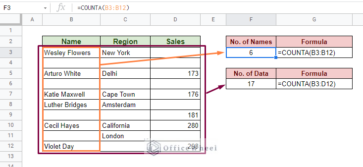
First up we have is the count. We will look to count all values in a range. In other words: Count all non-empty cells in the dataset or spreadsheet.
The COUNTA function is perfect for this scenario. Simply input the range within the function to count all cells with value.
For a single column:
=COUNTA(B3:B12)Multiple column formula:
=COUNTA(B3:D12)For an in-depth guide for this approach and more such scenarios, please see our Count Non-Empty Cells in Google Sheets article.
II. List All Cells with Value in One Column
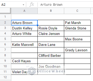
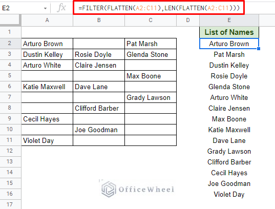
Here we have a list of names. We want to list all these names automatically. Meaning that we want to find and extract all cells that contain values in this dataset and place them in a column.
We have a simple formula to do so:
=FILTER(FLATTEN(A2:C11),LEN(FLATTEN(A2:C11)))The FLATTEN function combines all the values and presents them as a list (single column) on its own. However, that includes the blank cells in the range.
To remove these blank cells from the equation, we take the help of the FILTER and LEN functions.
3. Find and Highlight All Cells With Value in Google Sheets
Highlighting cells containing data is a common task for any spreadsheet professional. And it is mostly done by conditional formatting.
I. Highlight all Cells with Any Value (Non-Empty Cells)
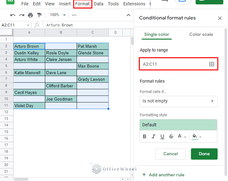
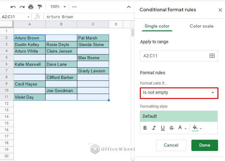
We start with something simple, which is to highlight all non-empty cells in our spreadsheet.
In the Conditional formatting rules window (Format tab > Conditional formatting), select the range of cells on which you want to apply conditional formatting.
The non-empty cells will be highlighted by default. If not, select the “Is not empty” option from the Format rules section.
II. Highlight all Cells with a Specific Value
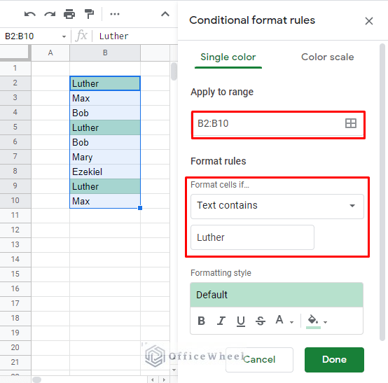
Similarly, we can find and highlight all cells that contain a specific text in Google Sheets using conditional formatting.
As before, we determine the range of cells first and then move to input the highlight condition. This time, our Format rules will have the Text contains option. We have selected the text “Luther” to highlight.
The formatting style is completely at the user’s discretion.
For a more in-depth guide to conditional formatting, please see our How to Use Conditional Formatting in Google Sheets article.
Read More: How to Create Conditional Drop Down List in Google Sheets
Final Words
That concludes all the ways you can use to find all cells with values in Google Sheets. The application is versatile enough to provide us with a solution for every scenario. We have the COUNTA function for any non-empty cell, LOOKUP functions for finding cells with specific values, and conditional formatting to highlight any cell with values.
Feel free to leave any queries or advice you might have for us in the comments section below.
Related Articles
- How to Use Find and Replace in Column in Google Sheets
- Easy Guide to Replace Formula with Value in Google Sheets
- Search in Google Spreadsheet (5 Easy Ways)
- How to Find Frequency in Google Sheets (2 Easy Methods)
- Find Trash in Google Sheets (with Quick Steps)
- Find and Replace with Wildcard in Google Sheets
- [Fixed!] INDEX MATCH Is Not Working in Google Sheets (5 Fixes)
- Alternative to Use VLOOKUP Function in Google Sheets

