Google Sheets allows us to perform searches for data and values in many different ways. So today, in this article we look at how to search in Google spreadsheet for various scenarios, with both technique and formulas.
Let’s get started.
5 Ways to Search in Google Sheets
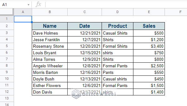
To present our processes today, we will be using the following dataset. It should cover the many different scenarios that people face in their day-to-day tasks.
1. Search with the Find Option (Keyboard Shortcut) in Google Sheets
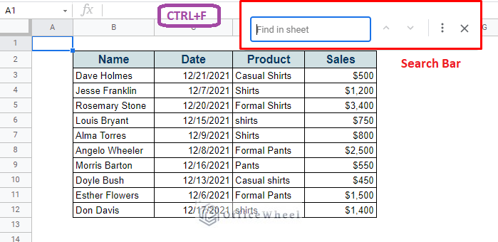
The first method we are going to discuss is the simplest and most basic, the Find option.
It is easily accessible with a keyboard shortcut:
- CTRL+F (Windows)
- CMD+F (Mac)
Which opens the Search Bar.
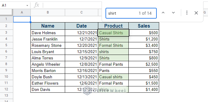
Inputting our search text, “shirt”, will highlight all the cells that contain this particular set of characters within the worksheet, regardless of case.
While this method does allow you to search for your desired text or number, search queries in a spreadsheet are not always that simple. The following methods will discuss varying scenarios that will utilize different types of search in a Google spreadsheet.
2. Search with the Find and Replace Option
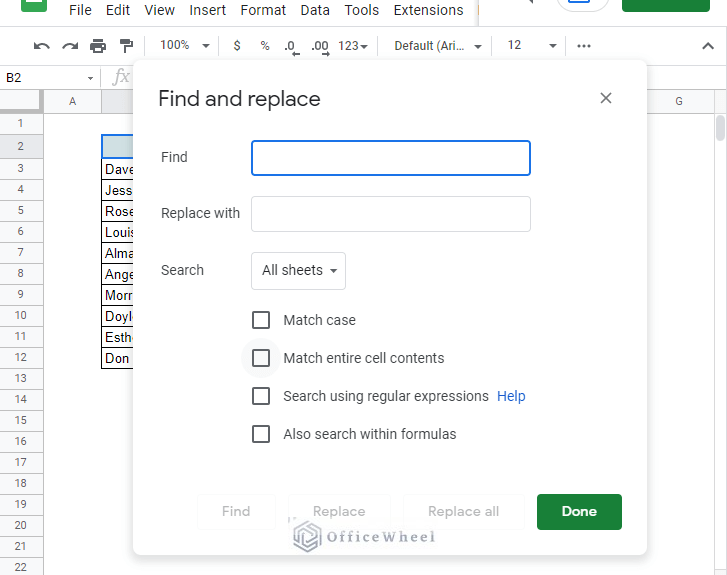
The next level to the Find option is the Find and Replace option of Google Sheets. This function not only searches for the given text but also goes the extra mile to find conditional queries and replace them if needed in one go.
You can navigate to Find and replace from the Edit tab on the top of the Toolbar.
Edit > Find and replace
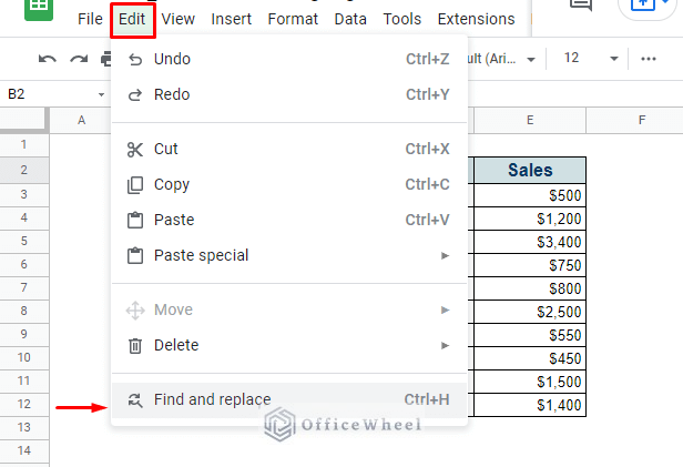
Or you can use the keyboard shortcut, CTRL+H, to open the Find and replace window.
To show the capabilities of this function, let’s find and replace all “shirts” that start with small “s” and replace them with “Shirts”.
Step 1: Open the Find and replace window.
Step 2: Search for “shirts”. Click Find. (this is optional)
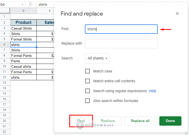
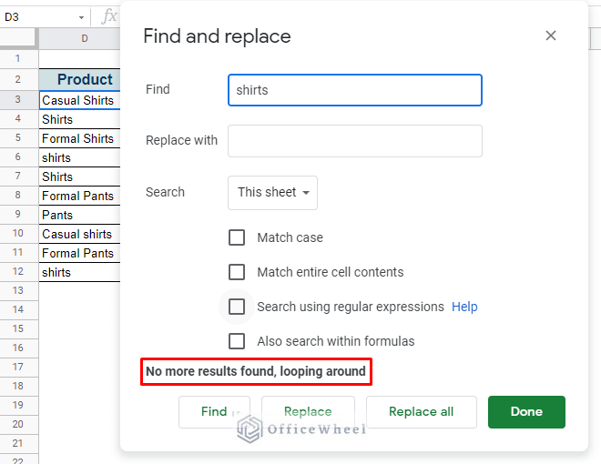
Keep clicking Find to see the different instances of the search query. Once all the instances have been found, the window will notify you with a message: No more results found, looping around.
Step 3: Apply the following conditions for our task:
- Find: shirts
- Replace: Shirts
- Search: This Sheet
- Check the Match case option
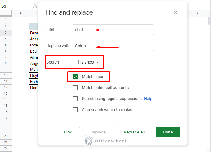
Step 4: Click Replace all.
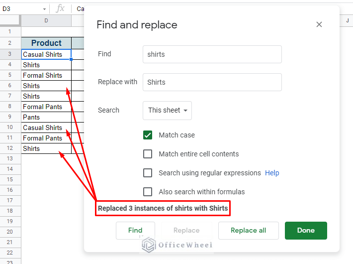
Rows 6, 10, and 12 have been updated.
What we have shown is only a small percentage of the capabilities of the Find and replace option, but this is the extent of it being utilized for basic search in a Google spreadsheet.
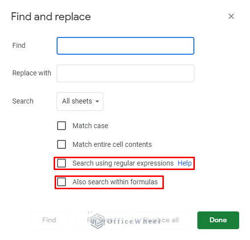
You can also search for formulas and specific string sequences with regular expressions with this option. Please see our Find and Replace in Google Sheets (3 Ways) article for an in-depth guide.
Read More: How to Use Find and Replace in Column in Google Sheets
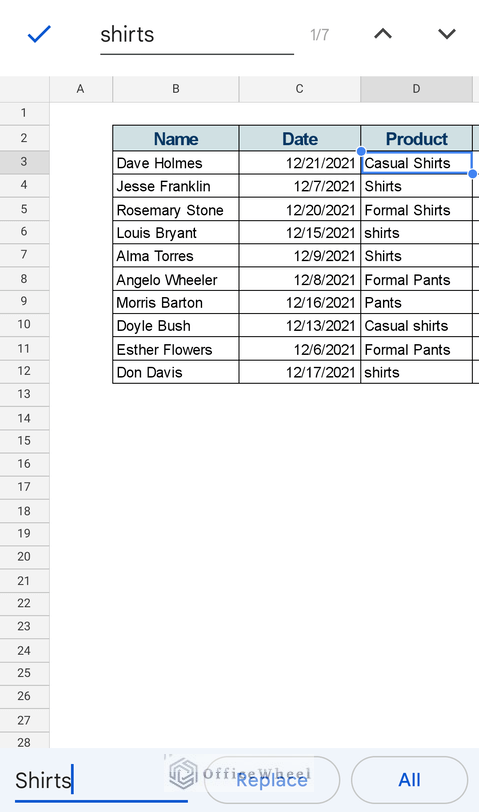
Find and Replace from a Mobile Device
We can also access Find and Replace from the mobile version of Google Sheets.
Tap the vertical 3-dots icon on the top-right corner of the screen to open the options menu.
Tap on Find and replace.
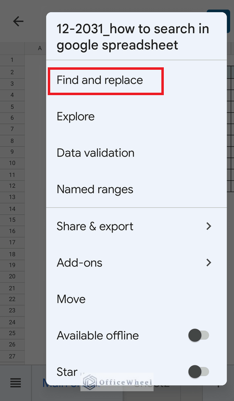
The Find and Replace option of the mobile device is limited to basic functions only.
Similar Readings
- Remove Characters from a String in Google Sheets (6 Easy Examples)
- How to Find Merged Cells in Google Sheets (3 Ways)
- How to Use the Find Function in Google Sheets (An Easy Guide)
- Substitute Multiple Values in Google Sheets (An Easy Guide)
- How to Remove Comma in Google Sheets (3 Easy Ways)
3. Search and Highlight using Conditional Formatting in Google Sheets
Conditional formatting is a fairly advanced way to search in a Google spreadsheet.
It combines the base search feature of the Find option, with the complex search options of Find and Replace, the ability to take custom formulas for searches, and finally, permanently highlight the searched values.
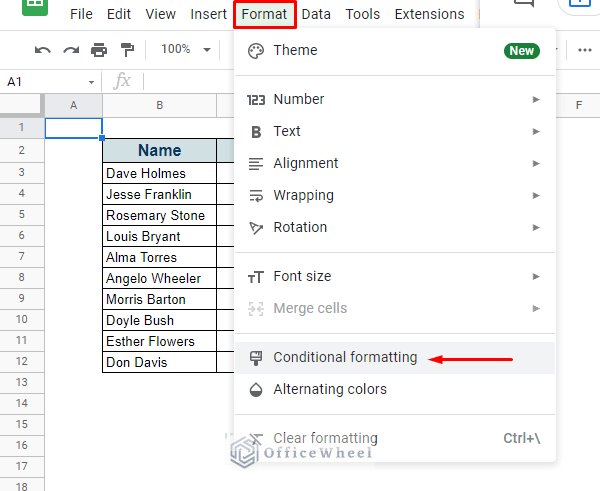
You can access the conditional formatting menu from the Format tab in the Toolbar.
Format > Conditional formatting
In the Conditional formatting rules menu, we have to apply certain conditions.
Step 1: Set the range. This is the range of cells that is to be counted and affected.
Step 2: Set the Format rules. We have chosen the Text contains option.
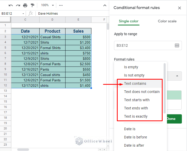
As you can see from the drop-down, there are a plethora of options to select according to your needs. Here are just the Text search options:
- Text contains: Highlight cells that contain given text.
- Text does not contain: Highlight cells that do not contain the given text.
- Text starts with: Highlight cells that start with the given text as value.
- Text ends with: Highlight cells the end with the given text as value.
- Text is exactly: Highlight cells that only contain the given text.
Step 3: Add the search keyword. We are looking for all the occurrences of “Shirts”
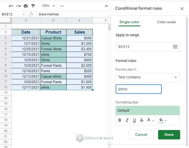
The main selling point of Conditional formatting is its ability to highlight cells according to complex conditions or criteria. This essence is captured by the Custom formula is option.
Here, we have highlighted rows that contain the word “Shirts” in the Product column.
The custom formula:
=$D3="Shirts"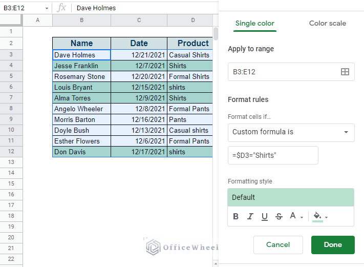
Our Conditional Formatting Based on Another Cell in Google Sheets article covers all methods in-depth on these custom formulas for conditional formatting.
Read More: Find Value in a Range in Google Sheets (3 Easy Ways)
4. Search using the QUERY function in Google Sheets
QUERY is a very powerful function of Google Sheets, especially when it comes to searching and extracting cells, rows, or columns that contain specific data.
The condition for our search query is to extract all rows of the table that have a Sales value greater than, let’s say, $1000.
Let’s through the query search process step-by-step:
Step 1: In the designated cell, for us, it’s cell B16, apply the QUERY function, =QUERY(.
Step 2: Select the range. We have selected the whole table including headers. Our range is B2:E12.
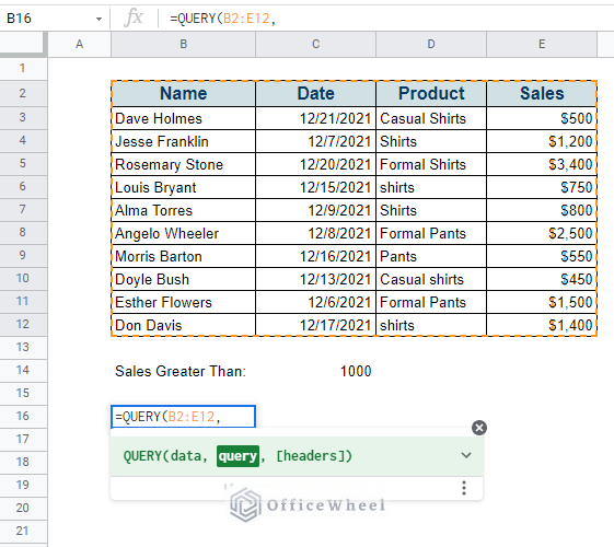
Step 3: We will now apply the query, which is “SELECT * WHERE E > 1000” (make sure that the query is enclosed in quotation marks). Then input 1 after comma (,) as we have included the table headers in our selection.
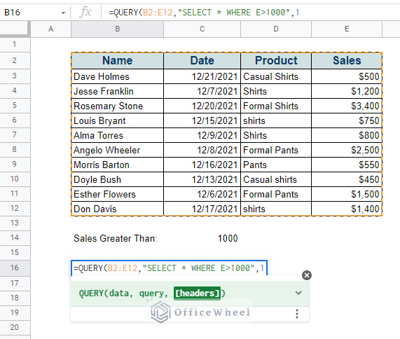
Step 4: Close parentheses and press ENTER.
=QUERY(B2:E12,"SELECT * WHERE E>1000",1)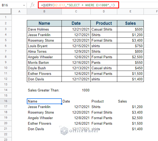
We can make the process slightly more dynamic by using a cell reference for our condition. You may have noticed our condition in cell C14.
To add this cell reference condition we have to concatenate the reference in-between the query with the ampersand (&) operator.
Our updated formula:
=QUERY(B2:E12,"SELECT * WHERE E>"&C14&"",1)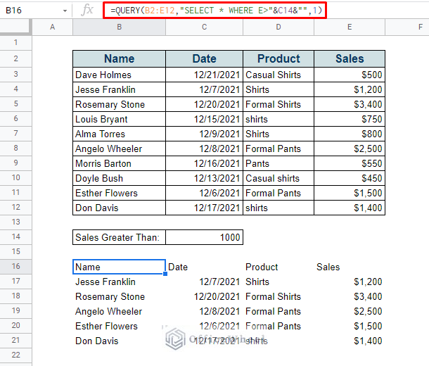
The QUERY formula in action:
Read More: How to Find the Range in Google Sheets (with Quick Steps)
5. Search for String within a Text in a Cell
For this method, we will be using the SEARCH function. SEARCH is a niche function used to find the location of a text within a cell.
Following our examples before, let’s use the SEARCH function to find the string “Shirt”. Our formula:
=SEARCH("Shirt",D3)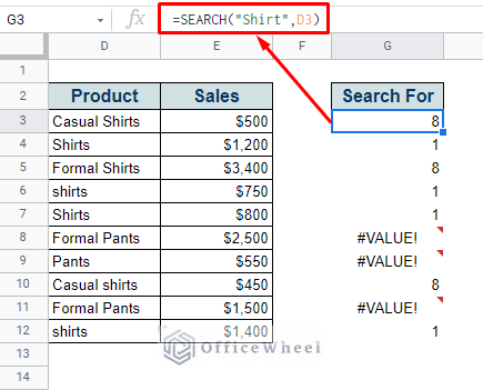
As we can see, the first value we get is 8. This is because the string “Shirt” starts from the 8th character, the whitespace is counted.
We also see a #VALUE error where the function failed to find any instance of the searched word.
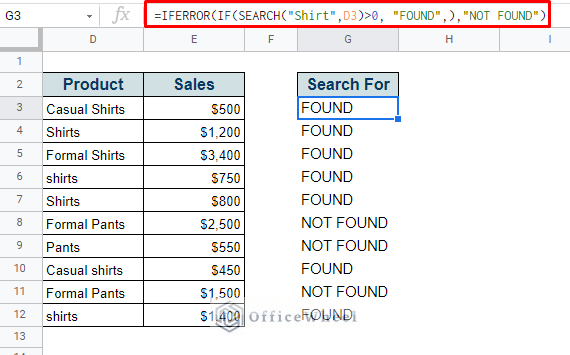
We can change our conditions to return as “FOUND” or “NOT FOUND” if the searched word exists in the cell.
Our new formula, which also takes the #VALUE error into account:
=IFERROR(IF(SEARCH("Shirt",D3)>0, "FOUND",),"NOT FOUND")Use the fill handle to apply to the rest of the column.
Read More: Find All Cells With Value in Google Sheets (An Easy Guide)
Final Words
We hope that all the methods we have discussed of how to search in a Google spreadsheet come in handy in your daily tasks.
Feel free to leave any queries or advice you might have for us in the comments section.
Related Articles
- How to Find and Delete in Google Sheets (An Easy Guide)
- Use FIND Function in Google Sheets (5 Useful Examples)
- How to Find P-Value in Google Sheets (With Quick Steps)
- Find and Replace with Wildcard in Google Sheets
- How to Find Hidden Rows in Google Sheets (2 Simple Ways)
- Find Largest Value in Column in Google Sheets (7 Ways)
- How to Find Correlation Coefficient in Google Sheets
- Find Uncertainty of Slope in Google Sheets (3 Quick Steps)