How to Find the Range in Google Sheets (with Quick Steps)

While working with large datasets it is sometimes hard to find and select the range. You can name the ranges in datasets and can find them easily. In this article, you will learn how to find the range in Google Sheets using their names and use them in formulas.

Step-by-Step Procedure to Find Range in Google Sheets

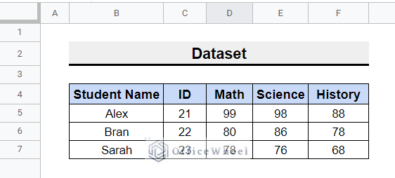
Let’s assume you have a dataset from obtained marks of students in different subjects. Now you need to find the ranges of numbers and use them in formulas to calculate total numbers, maximum and minimum obtained marks.

You can name the ranges in Google Sheets using the feature Named ranges so that you can find the ranges using their given names. The step-by-step procedure to find ranges in Google Sheets is given below.

Step 1: Name Columns and Rows Using Named Ranges Feature

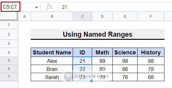
At the very beginning, you will need to name ranges using the Named ranges feature.

• To do this, first of all, select the range C5:C7.

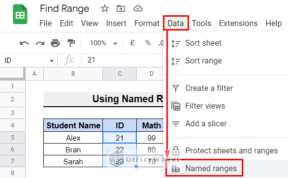
• Then, from the Google Sheets menu bar, select Data >> Named ranges.

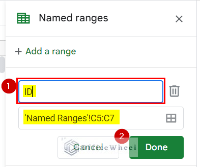
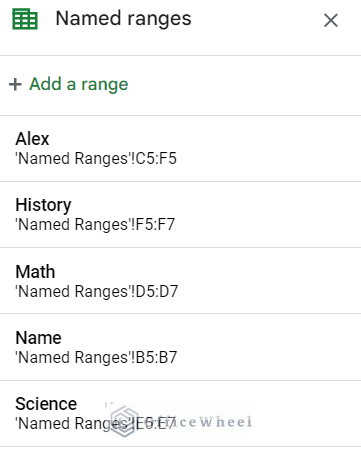
• Now, a pop-up box will appear. Here, to name the selected range enter ID in the first box. Then, press Done.

• Similarly, you can name other ranges in the dataset as well.

Read More: Find Value in a Range in Google Sheets (3 Easy Ways)

Similar Readings

• How to Search in Google Spreadsheet (5 Easy Ways)
• Remove Special Characters in Google Sheets (3 Easy Ways)
• How to Find and Delete in Google Sheets (An Easy Guide)
• Find and Replace with Wildcard in Google Sheets
• How to Use Find and Replace in Column in Google Sheets

Step 2: Use Named Ranges in Functions

Now, you can use and find these ranges to apply in functions.

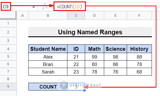
• For doing this, select cell C9 and enter the formula =COUNT(ID) to count the number of students and press Enter. The result of the formula will appear in the following screenshot.

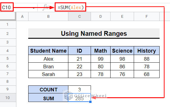
• Similarly, you can use the other named ranges in any formula to find the range and get your desired result.

Read More: Easy Guide to Replace Formula with Value in Google Sheets

How to Find Dynamic Named Ranges in Google Sheets

Dynamic named ranges are similar to named ranges, but the advantage of using this feature is that the formulas will automatically update as you add or remove one or more rows. You can do that in Google Sheets using the INDIRECT function.

Assume, you need to calculate the obtained number in History after entering the marks of another student. To calculate the total marks obtained in History after adding a further row, follow the steps below to create dynamic named ranges.

📌 Steps:

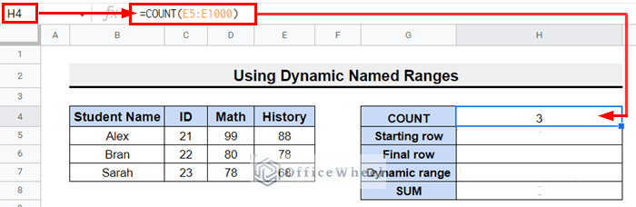
• First, select cell H4 and enter the formula =COUNT(E5:E1000) to count the data. The range E5:E1000 is used here to automatically count cells while a new row is entered.

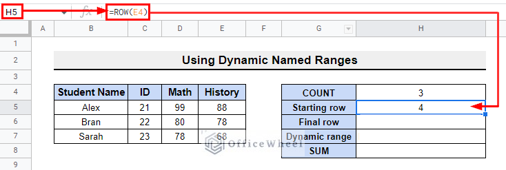
• Then, use the formula =ROW(E4) to count the starting row number.

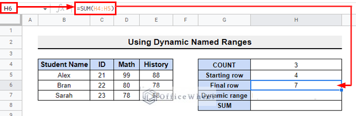
• Now, to count the final row, enter the formula =SUM(H4:H5).

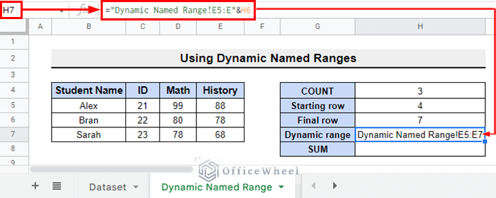
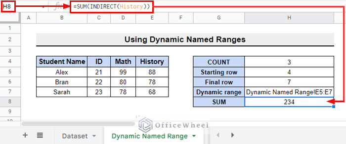
• Afterward, to create named range type formula, =”Dynamic Named Range!E5:E”&H6.

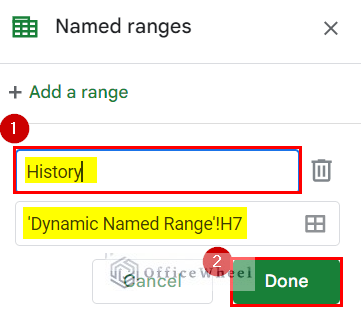
• After that, select cell H7 and go to Data>> Named ranges, then enter the range name History.

• Finally, to calculate the total obtained marks in History type formula =SUM(INDIRECT(History)) and the output will look like the following screenshot.

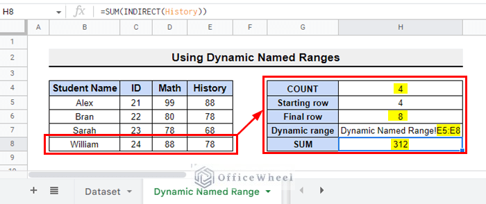
• Now if you add a new row, the sum of the obtained marks in History will be updated automatically.

Read More: How to Find Edit History in Google Sheets (4 Simple Ways)

Things to Remember

• Make sure that the cell references you are using are correct and that they refer to cells that contain data.

Conclusion

Hopefully, now you can find the range in Google Sheets using discussed step-by-step procedures. Please comment below with your doubts or suggestions regarding this article. Visit our website, OfficeWheel, for more articles on using functions.

Related Articles

• How to Find Hidden Rows in Google Sheets (2 Simple Ways)
• Find Slope of Trendline in Google Sheets (4 Simple Ways)
• How to Find Median in Google Sheets (2 Easy Ways)
• Find Uncertainty of Slope in Google Sheets (3 Quick Steps)
• How to Find Slope of Graph in Google Sheets (With Easy Steps)
• Find Frequency in Google Sheets (2 Easy Methods)
• How to Find Linear Regression in Google Sheets (3 Methods)