Nowadays, Google sheet is a very popular and widely used spreadsheet application. People are using this application because of the availability of the functions. The FIND function is one of the functions in Google Sheets and is widely used by users. In this article, we will demonstrate the anatomy of the FIND function. We will also highlight some examples of how to use the FIND function in Google Sheets. By the end of this article, you will know how to apply the function correctly in different cases.
A Sample of Practice Spreadsheet
You can download the practice spreadsheet from here.
What Is FIND Function in Google Sheets?
The FIND function returns the position of the first character of the string in the text. This function is case-sensitive.
Syntax
The syntax of the FIND function is as follows.
FIND(search_for, text_to_search, [starting_at])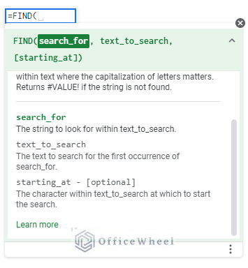
Arguments
| ARGUMENT | REQUIREMENT | FUNCTION |
|---|---|---|
| search_for | Required | The function looks for these characters within the string. |
| text_to_search | Required | In this string, the text searches for the first occurrence of search_for. |
| starting_at | Optional | The position to start the search from. |
Output
The formula FIND(“a”,”Here is a beautiful view”, 1) will return 9 as the first “a” of ”Here is a beautiful view” is in the 9th position.
5 Examples of Using FIND Function in Google Sheets
Let’s see the simple dataset below. In this dataset, we have some simple texts to demonstrate the use of the FIND function in Google Sheets with some practical examples.
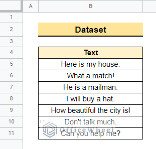
Follow the examples below to see how to apply the function.
1. Find Position of Specific Character
In this example, we will show how to get the exact position of a specific character using the FIND function. We will find the 1st occurrence of the Space (” “) character in this case. The steps are mentioned below.
📌 Steps:
- First, select cell C5 and insert the formula to get the actual position of a specific character.
=FIND(" ",B5)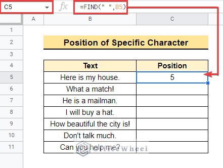
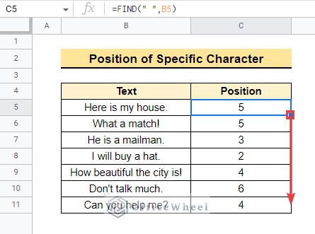
- After entering the formula drag down or double-click the fill handle to copy the same formula into the range C5:C11.
Read More: How to Find the Range in Google Sheets (with Quick Steps)
2. Find Position of Nth Occurrence of Character
Sometimes datasets may contain the same characters multiple times in a single string. Here we will find the 1st and 2nd occurrences of the same characters using the FIND function. Then you can apply the example to find the nth occurrence of any character in a string.
📌 Steps:
- First, we will find the 1st occurrence of the space character. We will insert the formula into cell C5.
=FIND(" ",B5)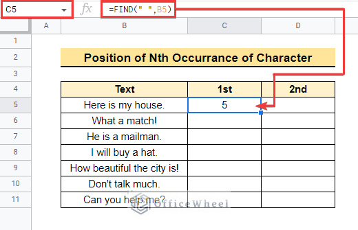
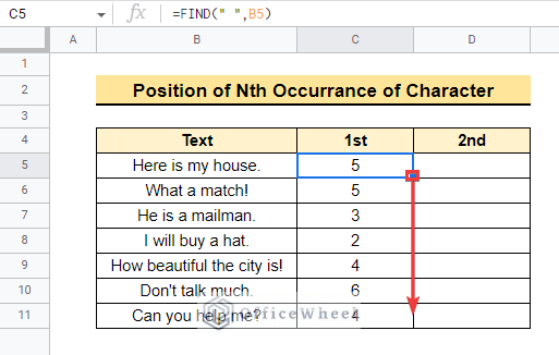
- Then we need to copy the formula down or double-click on the fill handle like before.
- Next, apply the following formula to cell D5 to get the 2nd occurrence of the character.
=FIND(" ",B5,FIND(" ",B5)+1)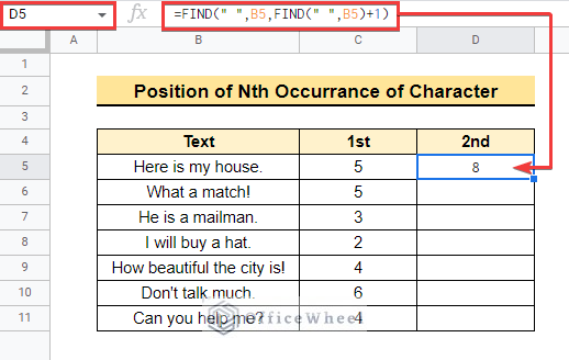
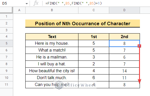
- Lastly, we will drag down the fill handle to copy the formula as shown below.
Formula Breakdown
➣ FIND(” “,B5): Here, the FIND(” “,B5) returns 5 i.e the position of the 1st occurrence of the character.
➣ FIND(” “,B5,FIND(” “,B5)+1): Here FIND(” “,B5)+1 returns 5+1 = 6. So the final formula becomes FIND(” “,B5,6). It finds the position of the space character starting from the 6th position.
Read More: Easy Guide to Replace Formula with Value in Google Sheets
3. Locate Case-Sensitive Characters
The FIND function is a case-sensitive function. Here, we will learn how to locate case-sensitive characters using the same dataset.
📌 Steps:
- In this case, we will find the position of “h” in the dataset. Select cell C5 and enter the formula below.
=FIND("h",B5)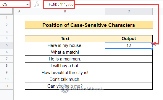
- After entering the formula we will drag down the fill handle like before to complete the process.
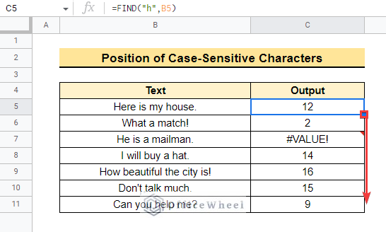
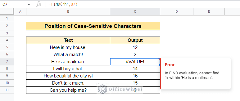
- Here, cell C7 shows #VALUE! because cell B7 does not contain any character “h” although cell B7 has the character “H”.
- As the FIND function is case-sensitive it will declare no match.
Read More: Find All Cells With Value in Google Sheets (An Easy Guide)
Similar Readings
- How to Search in Google Spreadsheet (5 Easy Ways)
- Find Uncertainty of Slope in Google Sheets (3 Quick Steps)
- How to Find Correlation Coefficient in Google Sheets
- Replace Space with Dash in Google Sheets (2 Ways)
- How to Convert Text to Date in Google Sheets (3 Easy Ways)
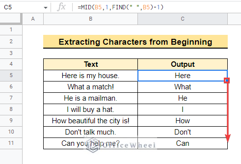
4. Extract Characters from Beginning of Strings
Now, we will learn how to extract characters from the beginning of the string using the FIND and MID functions. The MID function returns the characters from the middle of a string as this function is a text function. Here we will use the same Dataset as follows.
📌 Steps:
- At first, we select cell C5 and apply the formula below.
=MID(B5,1,FIND(" ",B5)-1)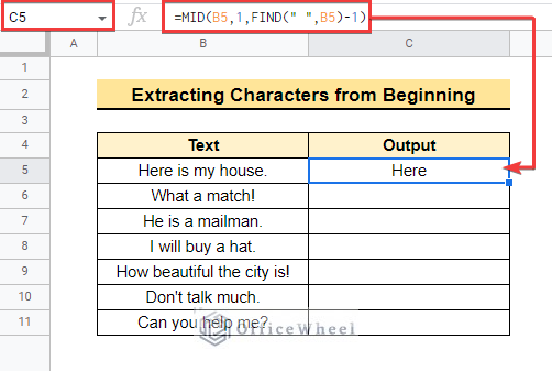
- Now, we will drag the formula down or double-click the fill handle icon to copy the formula below.
Formula Breakdown
➣ FIND(” “,B5)-1: Here, the FIND function returns 5 i.e. the 1st occurrence of the space character. So the final output is 5-1 = 4.
➣ MID(B5,1,FIND(” “,B5)-1): Here, the final formula becomes MID(B5,1,4). So the MID function returns 4 characters starting from 1.
Read More: How to Remove Characters from a String in Google Sheets (6 Easy Examples)
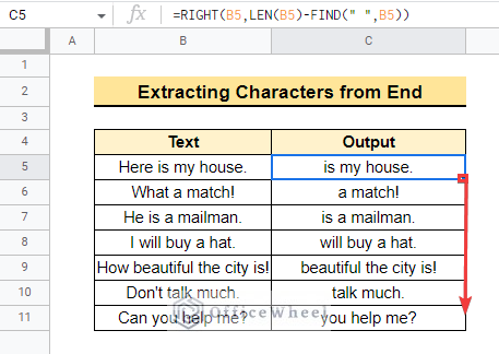
5. Get Characters from End of Strings
With the same dataset here, we will learn how to get characters from the end of the strings using the RIGHT, LEN, and FIND functions. Here, the RIGHT function returns a particular character from the end of the string, and the LEN function counts the total characters of a string.
📌 Steps:
- First, enter the following formula in cell C5 as shown in the following picture.
=RIGHT(B5,LEN(B5)-FIND(" ",B5))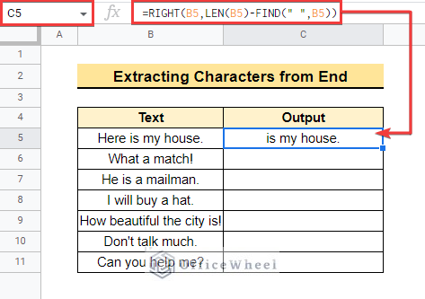
- Then drag down the fill handle to copy the same formula to the cells below.
Formula Breakdown
➣ FIND(” “,B5): Here, the FIND function will return the 1st occurrence of the space character (“ “). So the output will be 5.
➣ LEN(B5): Here, the LEN function returns the total number of characters in cell B5 i.e. 17. So LEN(B5)-FIND(” “,B5) returns 17 – 5 = 12.
➣ RIGHT(B5,LEN(B5)-FIND(” “,B5)): The final formula becomes RIGHT(B5,12). Then the RIGHT function extracts 12 characters from the right side of the string in cell B5.
Read More: How to Format Date with Formula in Google Sheets (3 Easy Ways)
What to Do When FIND Function Is Not Working in Google Sheets
The examples shown above suggest that the FIND function is extremely useful and we can use this function for many purposes. But sometimes it can give us problematic results. As the FIND function is case-sensitive, we can’t use this function when we use different cases.
- For example, the formula FIND(“h”,He is a mailman,1) in cell C7 returns #VALUE! Because it considers H as a mismatch to h.
=FIND("h",B7,1)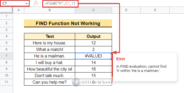
- In that case, we can use the SEARCH function as it is not case-sensitive. The output of the SEARCH function is shown in the following picture.
=SEARCH("h",B5,1)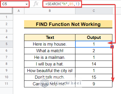
Things to Remember
- The FIND function is case-sensitive so we need to be careful while entering the formula.
- If there are multiple same characters in different positions, then the FIND function will return the position of the 1st character only.
Conclusion
In this article, we explained the anatomy of the FIND function. We also explained how to use the FIND function in Google Sheets with some useful examples. Hopefully, the methods will help you to apply the function to your own dataset. Please let us know in the comment section if you have any further queries or suggestions. You may also visit our OfficeWheel blog to explore more Google Sheets-related articles.
Related Articles
- How to Find Hidden Rows in Google Sheets (2 Simple Ways)
- Find Uncertainty of Slope in Google Sheets (3 Quick Steps)
- How to Find Median in Google Sheets (2 Easy Ways)
- Find Frequency in Google Sheets (2 Easy Methods)
- How to Find Edit History in Google Sheets (4 Simple Ways)
- Find Largest Value in Column in Google Sheets (7 Ways)
- How to Find Trash in Google Sheets (with Quick Steps)