[Solved!] VLOOKUP Function Is Not Working in Google Sheets

The VLOOKUP function is a dynamic tool in Google Sheets. We can search for any values in any given range with the help of this function. But sometimes you might find that the VLOOKUP function is not working in Google Sheets. In this article, I’ll discuss 8 easy fixes when the function is not working with clear images and steps.

A Sample of Practice Spreadsheet

You can download Google Sheets from here and practice very quickly.

8 Solutions When VLOOKUP Function Is Not Working in Google Sheets

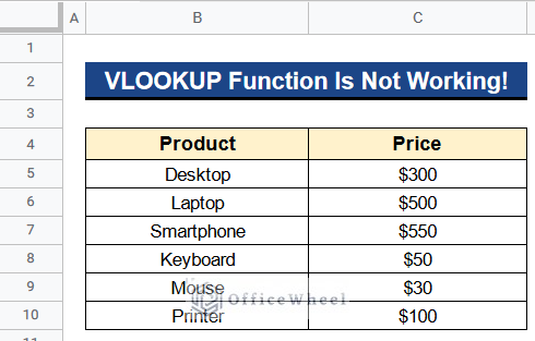
Let’s get introduced to our dataset first. Here we have some products in Column B and their prices in Column C. With the help of this dataset, I’ll show you 8 useful solutions when the VLOOKUP function is not working in Google Sheets.

Solution 1: Checking Delimiters

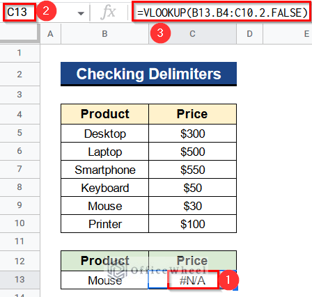
The delimiter is the sign we use when we enter any function in Google Sheets. Normally we use a comma (,) as our delimiters. Using wrong delimiters will give a #N/A Error. From our dataset, we want to look for the price of the Mouse. So, in our dataset, we have used this formula-

As we have used dot sign (.) as our delimiters the output is giving a #N/A Error. Let’s see how to correct it.

Steps:

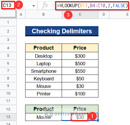
• Firstly, type the following formula with the right delimiters (,) in Cell C13–

• Then hit Enter to get the output.

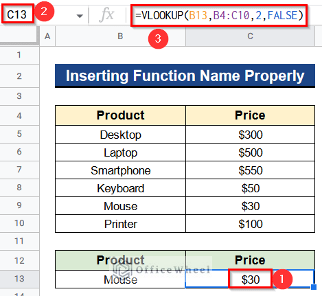
Solution 2: Inserting Function Name Properly

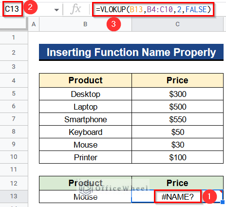
We have to put the function name properly to get the desired result. So, check for any spelling mistakes you may have made during applying the VLOOKUP function. In our dataset, we have put the formula shown below-

As we have done a spelling mistake it is giving a #NAME? error.

Steps:

• First, write the next formula in Cell C13–

• Next, press Enter to get the result correctly.

Solution 3: Giving Cell Reference Correctly

Giving correct cell references is also important during applying the VLOOKUP function. A cell reference is a value that the function searches within the given range of data. Like in this case we have given Cell E6 as a reference whereas our desired value is in Cell B13. That’s why applying the formula will give a #N/A Error–

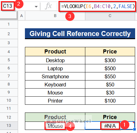
Steps:

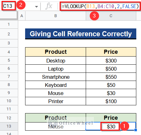
• First of all, insert the below formula in Cell C13–

• After, hit the Enter Button to get the correct output.

Read More: Highlight Cell If Value Exists in Another Column in Google Sheets

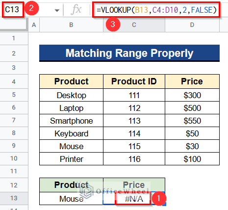
Solution 4: Matching Range Properly

You should also put the data range correctly in the VLOOKUP function. Otherwise, it’ll give a #N/A Error. Like in this case we have a new column titled Product ID in Column C. So, the prices are moved to Column D. Then when we apply the following formula it is giving an error-

It is giving an error because the function searches for the value Mouse in the range from Cell C4 to D10 which is the false range. Because VLOOKUP always searches through the first column of the range. Let’s correct it.

Steps:

• In the first place, put the formula in Cell C13–

• After that, press the Enter Button to get the result instantly.

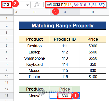
• Don’t forget to put the correct column index number which is 3 because we have our prices in column no 3 of our data range.

Read More: How to VLOOKUP All Matches in Google Sheets (2 Approaches)

Similar Readings

• VLOOKUP Error in Google Sheets (with Quick Solutions)
• How to VLOOKUP Between Two Google Sheets (2 Ideal Examples)
• Use IFERROR with VLOOKUP Function in Google Sheets
• How to Use VLOOKUP Function for Exact Match in Google Sheets
• VLOOKUP with Multiple Criteria in Google Sheets

Solution 5: Inserting Correct Column Index Number

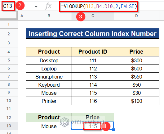
If we insert the wrong column index number then the VLOOKUP function will return the wrong value in Google Sheets. Like in our case we have inserted the formula like this-

The formula is returning the product id of the product but we want the price of the product. As we have put the column index no 2 it is giving values from column no 2, Column C.

Steps:

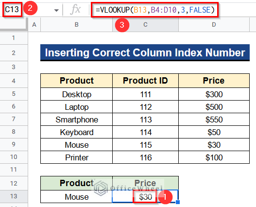
• In the beginning, type the following formula in Cell C13 with the correct column index no 3-

• Thereafter, hit Enter to get the output.

Read More: How to VLOOKUP Multiple Columns in Google Sheets (3 Ways)

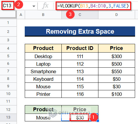
Solution 6: Removing Extra Space

We may have some extra spaces in our lookup value. Then the VLOOKUP function won’t work. Below the formula isn’t working because we have some spaces in Cell B13 as shown in the picture. We have applied the next formula and it isn’t working for having space in the value-

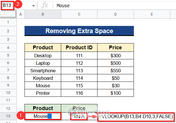
6.1. Manually Removing Space

We can remove the space manually like below.

Steps:

• Before all, write the next formula in Cell C13 after removing spaces from Cell B13–

• Afterward, press Enter to get the price.

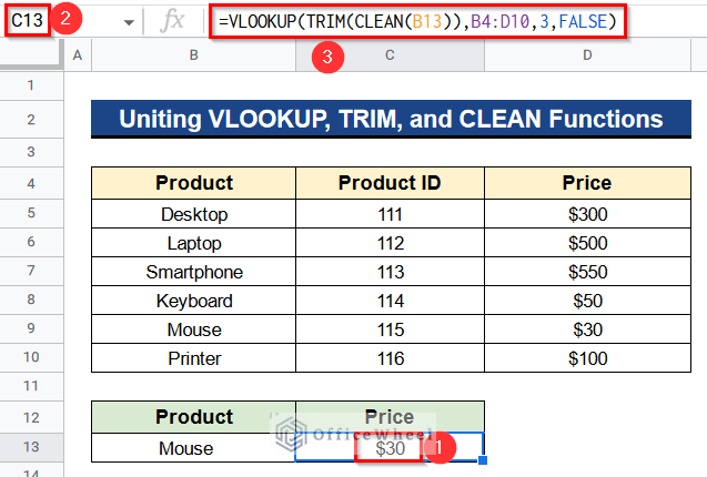
6.2. Uniting VLOOKUP, TRIM, and CLEAN Functions

Moreover, we can merge the VLOOKUP, TRIM, and, CLEAN functions to get results instantly. In this case, we don’t have to manually remove any space. The output is very fast.

Steps:

• Earlier on, insert the formula in Cell C13–

• Consequently, click Enter to get the desired output.

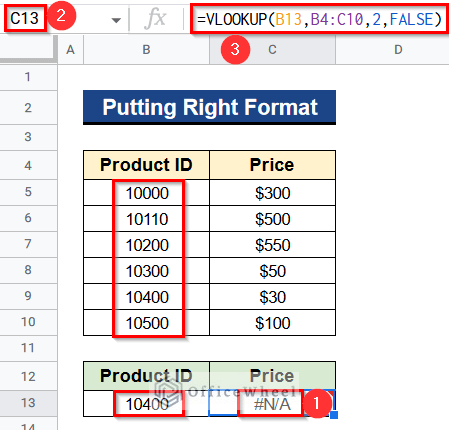
Solution 7: Putting Right Format

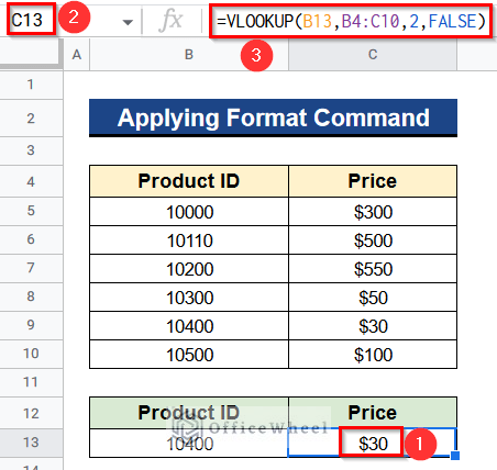
When we search for something with the VLOOKUP function the format should be similar for both value and dataset. Otherwise, we don’t get any results. Now in our dataset, we have product ids in text format but our given value in Cell B13 is in number format. So our next formula isn’t working here-

So we have to put a similar format when the VLOOKUP function is not working with the text format.

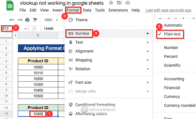
7.1. Applying Format Command

We can do this simply by applying the Format Command.

Steps:

• Initially, Select Cell B13 and go to Format > Number > Plain Text.

• Again, put the formula in Cell C13–

• Moreover, hit the Enter button to get the desired price.

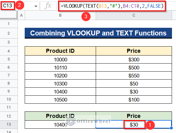
7.2. Combining VLOOKUP and TEXT Functions

Additionally, we can combine the VLOOKUP and TEXT functions to get the result instantly.

Steps:

• Before, type the following formula in Cell C13–

• After, click the Enter button to get the result.

Read More: Combine VLOOKUP and HLOOKUP Functions in Google Sheets

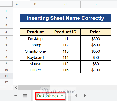
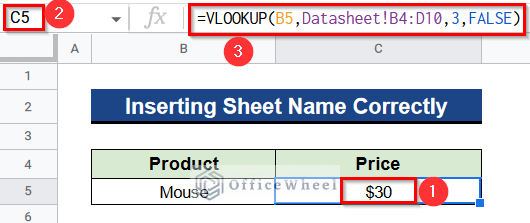
Solution 8: Inserting Sheet Name Correctly

Sometimes the VLOOKUP function does not work between sheets. We have a dataset like below which have products in Column B, their ids in Column C, and prices in Column D. We gave a name to our dataset which is Datasheet.

When we move to another sheet and apply the following formula it gives an #REF Error–

This error occurs because here we put the sheet name wrong.

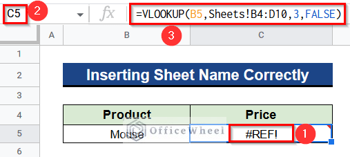
Steps:

• Firstly, type the following formula in Cell C13 with the correct sheet name-

• Finally, hit Enter to get the output instantly.

Read More: How to Use VLOOKUP with Named Range in Google Sheets

Conclusion

That’s all for now. Thank you for reading this article. In this article, I have discussed 8 easy solutions when the VLOOKUP function is not working in Google Sheets. Please comment in the comment section if you have any queries about this article. You will also find different articles related to google sheets on our officewheel.com. Visit the site and explore more.

Related Articles

• Google Sheets Vlookup Dynamic Range
• How to Use Wildcard in Google Sheets (3 Practical Examples)
• Use Nested VLOOKUP in Google Sheets
• How to Check If Value Exists in Range in Google Sheets (4 Ways)
• [Fixed!] Google Sheets If VLOOKUP Not Found (3 Suitable Solutions)
• How to VLOOKUP for Partial Match in Google Sheets
• 2 Helpful Examples to VLOOKUP by Date in Google Sheets
• How to Use VLOOKUP with Drop Down List in Google Sheets