Pull Data From Another Sheet Based on Criteria in Google Sheets (3 Ways)

No matter how much of an expert you are, many still sometimes find it difficult to extract data from one worksheet to another. Exponentially so when conditions and criteria are involved.

Today, in this article, we have broken down three processes we believe through which you can pull data from another sheet in Google Sheets quite easily.

Let’s have a look.

3 Ways to Pull Data From Another Sheet Based on Criteria in Google Sheets

1. Using the FILTER Function to Pull Data From Another Sheet

Let’s start with the simplest method to understand, which is using the FILTER function. What the FILTER function does is that it imports the entirety of the selected range based on the given criteria.

Filter function syntax:

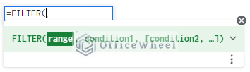
• range: The range of data that will be included in the data pull
• condition1: The first, or only, range of condition criteria that the data pull will follow
• [condition2, …]: More criteria can be added (optional)

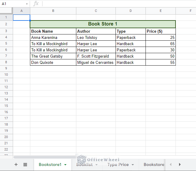
For this method, our objective is to populate the Booklist worksheet according to the book data available in another worksheet, Bookstore1. Our condition or criteria of the data pull is that we are only looking for Hardback books.

Step 1: We start at the Booklist worksheet. Here, in our first cell of the table, we type in the function:

This opens an in-cell prompt asking for range and conditions.

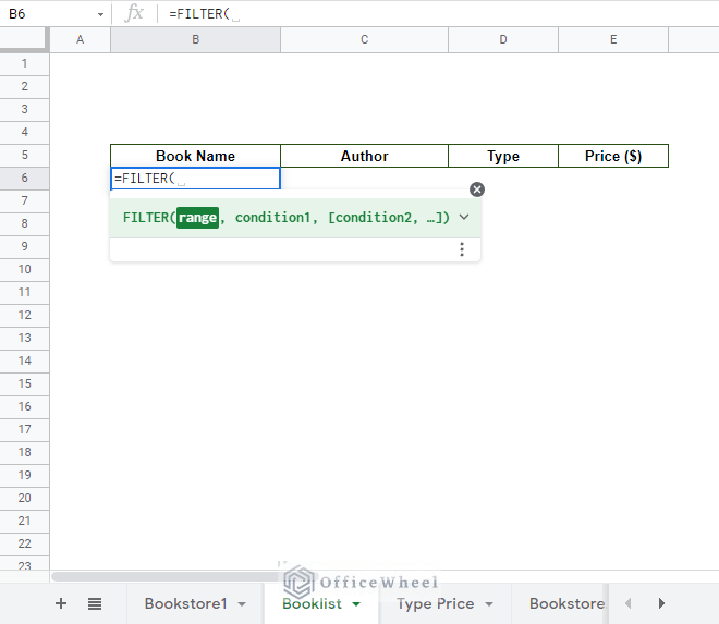
Step 2: We move to our desired worksheet, Booklist1 in our case, and select the range of data that we want to extract. We have selected all the data in this table, except the headers. You can drag your mouse across the table to select the data. Press comma (,) after you are done selecting the range.

Step 3: Select the condition column or range. In our case, it is the data under the Type column header.

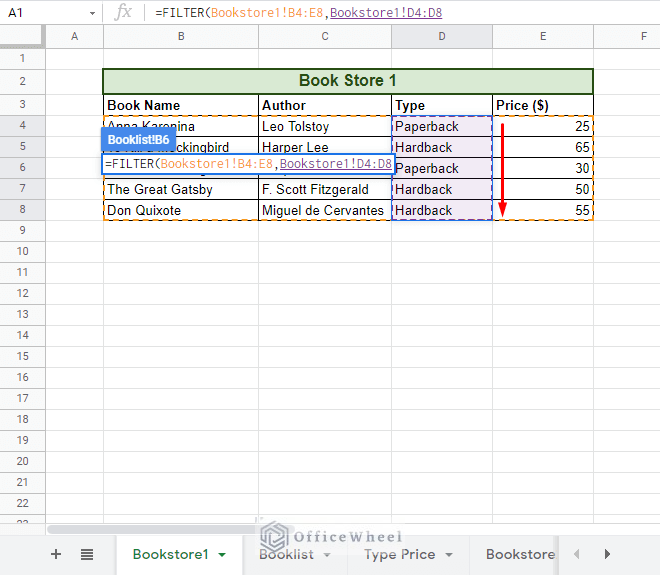
Step 4: We now have to add a condition to check. We are only checking for Hardback covers. So, after the condition range, we type =“Hardback”.

Note: We have added the quotations to show that our condition is of the text type. For number type conditions we do not use quotation marks.

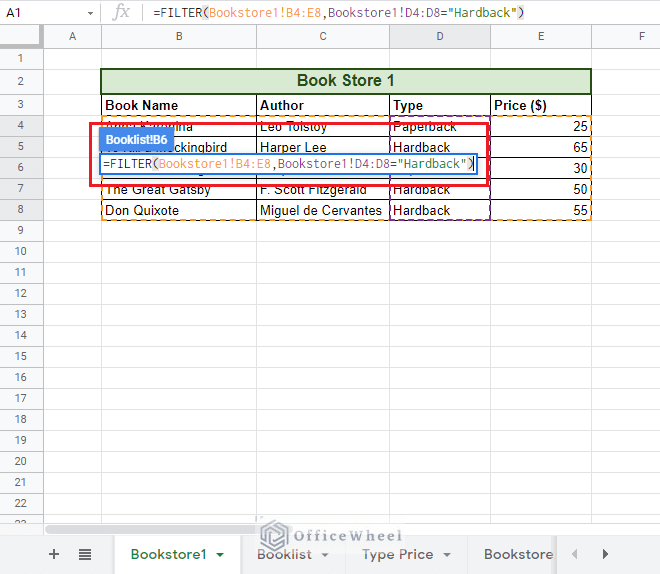
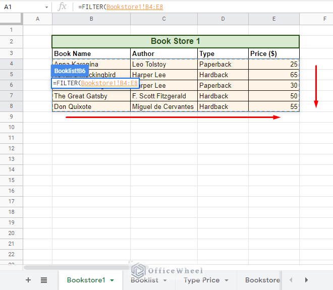
Step 5: Close parentheses and press ENTER. The list of books that have a hardback cover has been extracted to the Booklist worksheet.

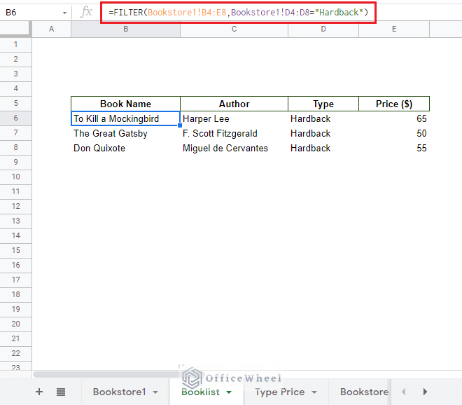
Extra Steps (Optional)

Let us take this opportunity to clean up and organize our Booklist worksheet a bit.

First of all, instead of writing down our condition every time we need or change something, let us use cell references to get it done.

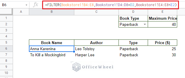
We have added the Book Type section above our Booklist table, here we have added the condition Hardback, in cell D2. We will be referring to this cell in our formula:

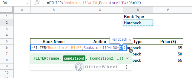
With this, you do not have to worry about the type of data you input.

Second, we will be adding the other book type, Paperback, to our condition. We will do this by adding a drop-down list in cell D2.

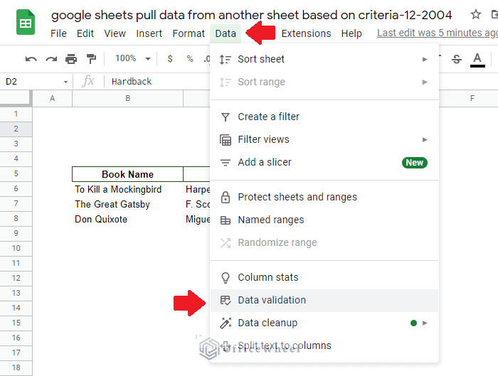
Step 1: Select the cell where you want the drop-down to be. It is cell D2 in our case.

Step 2: Navigate to the Data tab and select the Data Validation option.

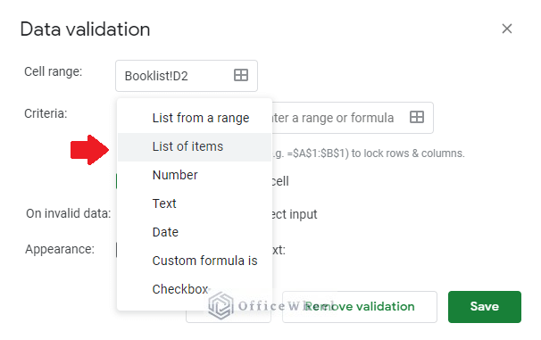
Step 3: In the Data Validation window select Criteria: List of Items.

Step 4: Add the drop-down options. Ours is Hardback and Paperback. Then check the Reject input radio button.

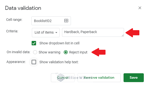
Step 5: Click Save

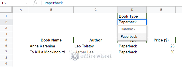
We had some fun and added an extra condition to our FILTER function. You can try something similar yourself.

Great! We have successfully pulled data from another sheet in Google Sheets using the Filter function.

Read More: Reference Another Sheet in Google Sheets (4 Easy Ways)

2. Using VLOOKUP to Pull Data From Another Sheet

Next, we will look at one of the oldest functions used for data extraction, the VLOOKUP function.

The syntax for the VLOOKUP function is:

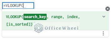
• search_key: The conditional data reference, the value to search for
• range: the range of the dataset where the function will find the value in search_key
• index: The number of the column (column index) from which value will be returned
• [is_sorted]: Indication of whether the column the function searches are sorted or not. This value is optional and by default it is TRUE.

Using the VLOOKUP function we can search a range of data in another worksheet to return a conditional value from the indicated column.

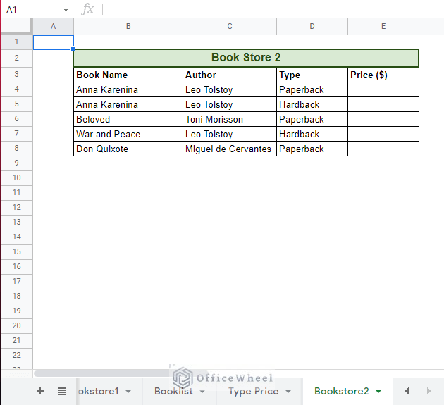
To break the usage of this function down, we have created two new worksheets. The Bookstore2 worksheet contains the information of the available books, and the Type Price worksheet contains the table of prices for each type of book cover.

The Step-By-Step Process

Using the VLOOKUP function we will be pulling data from the Type Price worksheet and populating the Price column of the Bookstore2 worksheet.

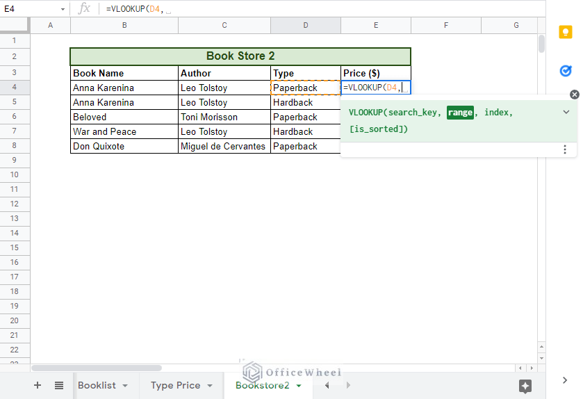
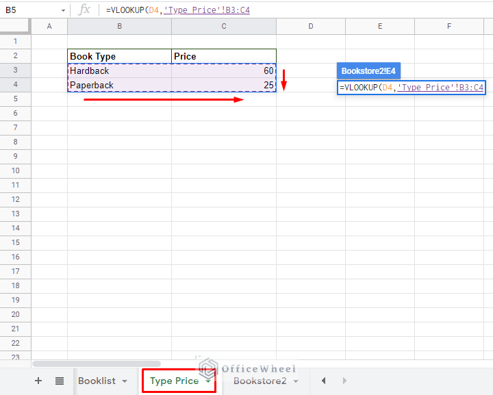
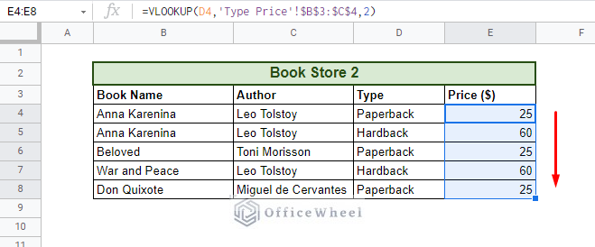
Step 1: We will be entering our formula in the first cell of the Price column. Here, type =VLOOKUP( and for the search_key we will be referring to the Type of book, in other words, cell D4. Press comma (,) after you are done selecting the key.

Step 2: We will now move on to the Type Price worksheet. Here, we will be selecting the range of data for our lookup value.

Step 3: Our desired return value, Price, is in the second column of the selected range. This our index value will be 2.

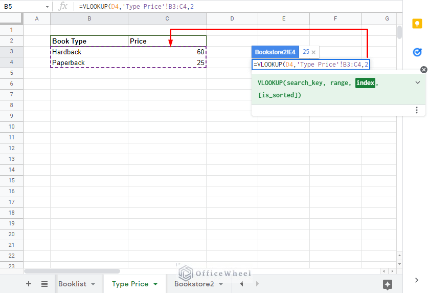
Step 4: Close the parentheses and press ENTER. We have successfully extracted the price data from a different worksheet.

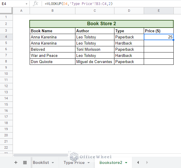
But it does not end here! To cover the rest of the column, we have to lock the range cell references, otherwise, we will be getting an error.

Step 5: Double click on cell E4 or use the formula bar to highlight the range section of the VLOOKUP function. Press the F4 key of your keyboard once, this will lock the cell reference in place (a dollar sign ($) will appear before the cell references indicating this). Press ENTER.

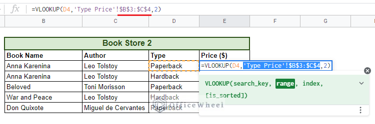
Note: We have just transformed the range cell reference to an Absolute Cell Reference.

Step 6: Use the fill handle to apply the formula to the rest of the column.

We have successfully used the VLOOKUP function to pull data from another sheet in Google Sheets!

Read More: Return Cell Reference in Google Sheets (4 Easy Ways)

Similar Readings

• Reference Cell in Another Sheet in Google Sheets (3 Ways)
• Conditional Formatting Based on Another Cell in Google Sheets

3. Using the QUERY Function to Pull Data From Another Sheet

A new and highly underrated function that Google Sheets has in its arsenal is the QUERY function.

The syntax of the Query function is:

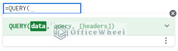
• data: The range of cells that you want to perform the query on. It can cover the entire worksheet in a pinch if we give the range A:Z.
• query: The query that you want to perform. The query must be enclosed in quotation marks (“”).
• [headers]: Optional. Indicates the number of header rows above the desired data. Default: -1.

The QUERY function looks through the range designated by the data and applies the given query (condition/criteria) to them and returns the row values.

It may not cover all the bases as the FILTER function, like multiple criteria, but QUERY can save a lot of time if you have single or short queries.

For this method, we will be performing a similar process to that of method 1 of our article, but this time with the QUERY function instead of the FILTER function. We will be populating the second booklist in the worksheet Booklist2 with data taken from the Bookstore2 worksheet.

Step 1: Select the cell where you want to paste your query and type =QUERY(.

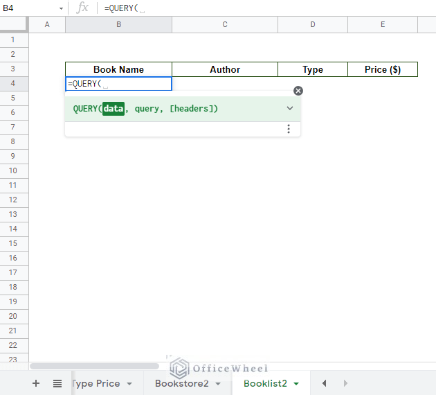
Step 2: Move to the other worksheet, Bookstore2 in our case, and select the data range.

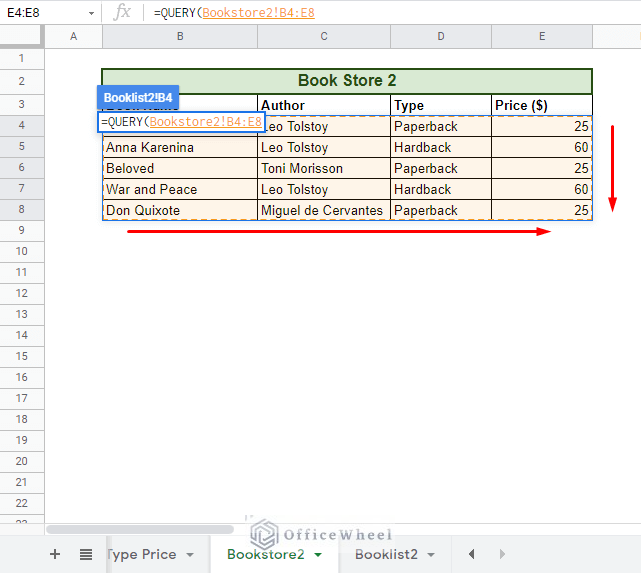
Step 3: Enter the criteria/condition/query. Remember to type your query within quotation marks (“”).

Our query is “where D = ‘Hardback'”, as we are looking to extract any rows that have the book cover type hardback in it.

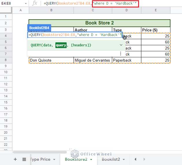
Step 4: Close parentheses and press ENTER.

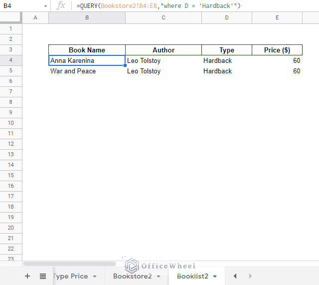
And that’s that! We have successfully pulled data from another sheet using the QUERY function.

Read More: How to Query Cell Reference in Google Sheets

Final Words

That is all we have for today. We hope that all of these functions utilized in various situations for different criteria will help you manage your data. If you have any other queries or advice for us, feel free to ask in the comment section.

Related Articles

• Reference Another Workbook in Google Sheets (Step-by-Step)
• Lock Cell Reference in Google Sheets (3 Ways)
• Indirect Sheet Name in Google Sheets (Easy Steps)
• Google Sheets: Use Cell Value in a Formula (2 Ways)
• Dynamic Cell Reference in Google Sheets (Easy Examples)
• Variable Cell Reference in Google Sheets (3 Examples)
• Reference Another Tab in Google Sheets (2 Examples)