We heard the term “Calculus”, didn’t we? One of the most important branches of mathematics. Not only in calculus but also in geometry, we need the basics of “slope” also known as “gradient”. Understanding those then applying it through Google Sheets or Excel is a smart idea for the best purposes right? In this article, we have demonstrated the easy step-by-step process to find the slope of a graph in Google Sheets.
A Sample of Practice Spreadsheet
You can download the spreadsheet used for describing methods for this article from here.
What is Slope?
The tangent (trigonometric operator “tan”) of the angle produced by a linear line with the positive X axis in the coordinate system is called slope or gradient of that linear line. The general equation of a straight line is-
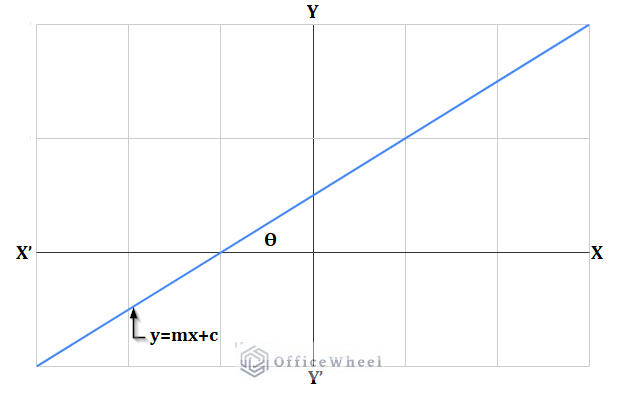
Here, m=tanθ; θ= angle with a positive X-axis produced by the linear line.
Step-by-Step Process to Find Slope of Graph in Google Sheets
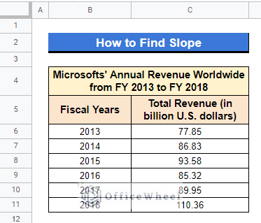
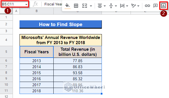
We will be using the following dataset as an example to find the slope of the graph in Google Sheets. The dataset represents Microsofts’ Annual Revenue Worldwide from FY 2013 to FY 2018.
Step 1. Create a Chart
- First, select Cell range B5:C11, next select Insert at the toolbar, and choose Chart.
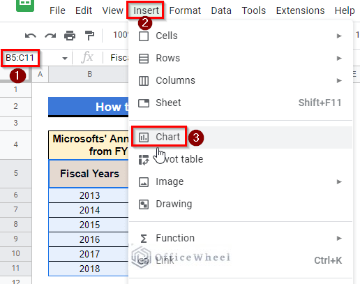
- Or simply left-click on the Insert chart ribbon from the toolbar.
Read More: Find Value in a Range in Google Sheets (3 Easy Ways)
Step 2. Open Chart Editor
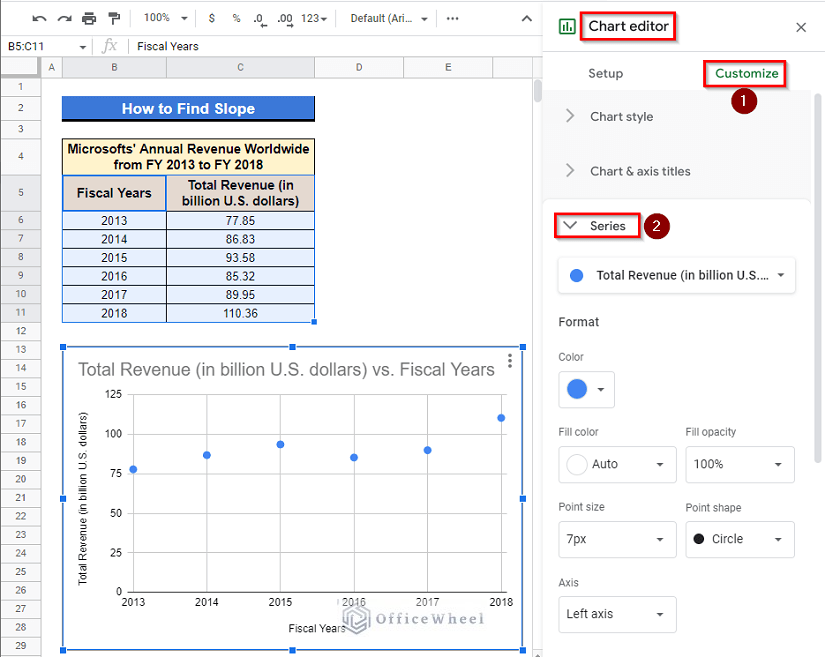
- After that, a chart will appear on your screen. But that one is not gonna help us with what we are looking for. Along with the chart, a sidebar titled Chart editor will also come up. Select Customize from there, pick drop down menu Series.
Step 3. Display Equation on Chart
- Mark the Trendline box and then from the Label drop down menu select the Use Equation option.
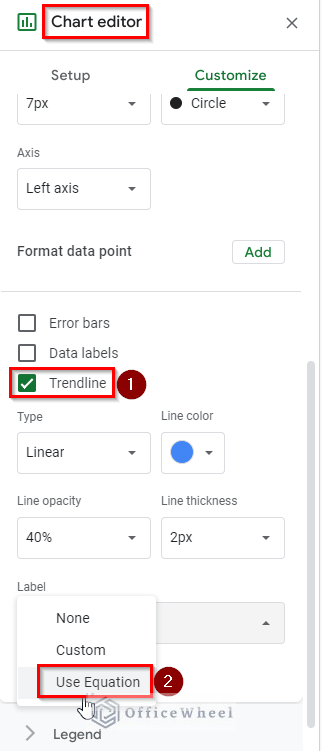
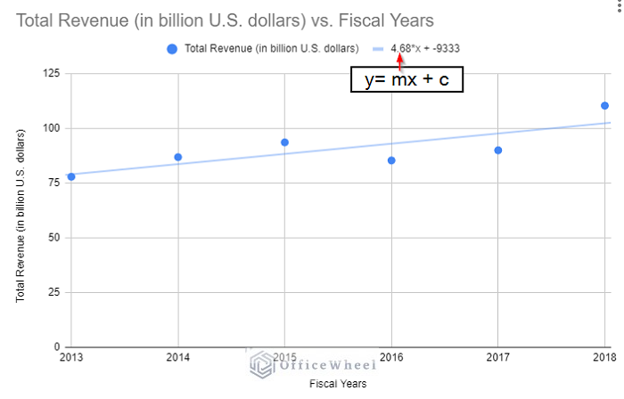
- Following this, you will find a linear equation that will appear on your chart.
Read More: How to Find Slope of Trendline in Google Sheets (4 Simple Ways)
Step 4. Get Slope by Comparing Equation on Chart
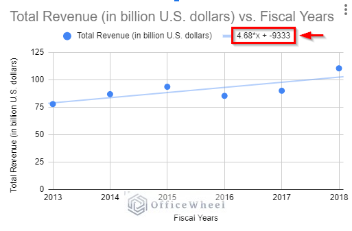
- Now, compare this equation with the general linear equation y=mx+c. What do you think? Obviously, the value of m is 4.68 which represents the value of the slope.

Similar Readings
- How to Find and Delete in Google Sheets (An Easy Guide)
- Use FIND Function in Google Sheets (5 Useful Examples)
- How to Use Find and Replace in Column in Google Sheets
- Find and Replace with Wildcard in Google Sheets
8 Ways to Find Slope Without Graph in Google Sheets
Previously we have seen how to find the slope of a graph using a chart in Google Sheets. But there are more methods to find the slope for a linear line. Here, we have described 8 alternatives to find the slope without a graph in Google Sheets. We will be using the same dataset for these as well as we have used for the previous one.
1. Using SLOPE Function
The SLOPE function in Google Sheets helps to find the gradient of two different given arrays. A linear equation basically represents the relationship between two variables where one is dependent and the other one is independent and both of the variables are either with power 1 or 0 (one variable must have power 1).
Steps:
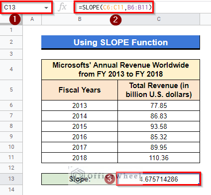
- In the following dataset, first select Cell C13, apply the following formula and press Enter–
=SLOPE(C6:C11,B6:B11)Here, Cell range C6:C11 contains the values of dependent variable Y and Cell range B6:B11 contains the values of independent variable X. The output will be visible in Cell C13 after applying the formula.
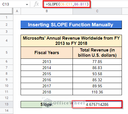
2. Inserting SLOPE Function Manually
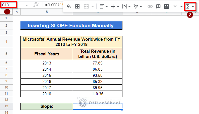
Except for typing down a formula, we can also calculate the slope of two data ranges using the built-in SLOPE function manually.
Steps:
- At first, select Cell C13, then at the toolbar, choose the Functions menu.
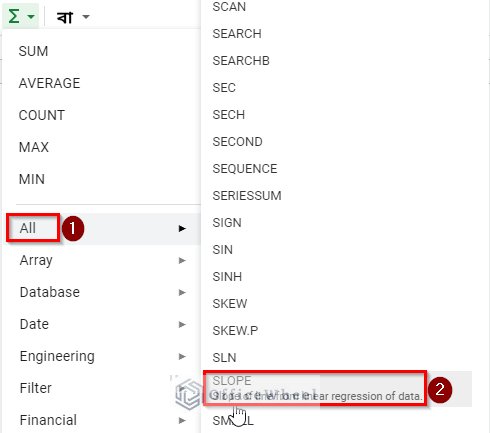
- From the menu, choose All and after that select SLOPE.
- You will be asked for the inputs.
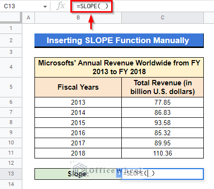
- First, select Cell range C6:C11 then a comma, and then select Cell range B6:B11, finally press Enter to see the result.
Here Cell range C6:C11 indicates the values of dependent variable Y and Cell range B6:B11 represents the values of independent variable X.
Read More: How to Find the Range in Google Sheets (with Quick Steps)
3. Employing TREND Function
The TREND function is an additional function that can be used to determine the slope. Additionally, depending on a predetermined value for the independent variable, it returns the expected value of the dependent variable in the future.
Steps:
- Select Cell C13 in the following dataset, apply the formula below and press Enter–
=TREND(C6:C11,B6:B11,1,true)-TREND(C6:C11,B6:B11,0,true)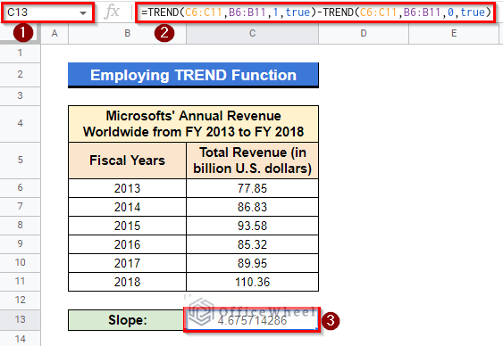
Formula Breakdown
- TREND(C6:C11,B6:B11,1,true)
Here, this formula basically returns the value of m+c (slope+Y-axis intercept).
- TREND(C6:C11,B6:B11,1,true)-TREND(C6:C11,B6:B11,0,true)
The second TREND function here returns the value of “c” only. Further, the whole function calculates (m+c-c) and returns only “m”.
Read More: Find All Cells With Value in Google Sheets (An Easy Guide)
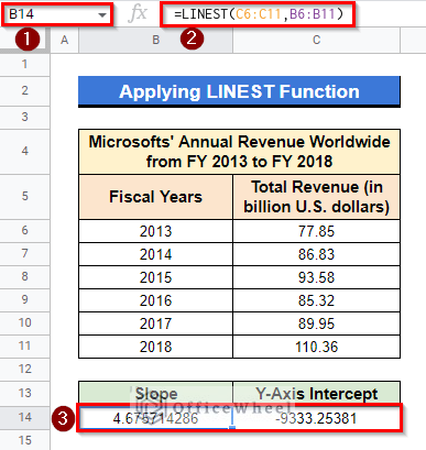
4. Applying LINEST Function
The LINEST Function returns both values of slope and Y-intercepts of a linear equation. As I have shown earlier, the equation of linear line y=mx+c, m & c are the slope and Y-axis intercept respectively. The LINEST function returns the values of these two.
Steps:
- First, select Cell B14 and apply the following formula below then press Enter–
=LINEST(C6:C11,B6:B11)- The value of slope “m” will appear on Cell B14 and the value of “c”, that is Y-intercept will return in Cell C14.
Read More: Easy Guide to Replace Formula with Value in Google Sheets
5. Embedding FORECAST Function
In order to establish the linear relationship between value series and timeline series, Google Sheets’ FORECAST function uses linear regression to forecast future values.
Steps:
- Provide the following formula after activating Cell C13 and then press Enter-
=FORECAST(1,C6:C11,B6:B11)-FORECAST(0,C6:C11,B6:B11)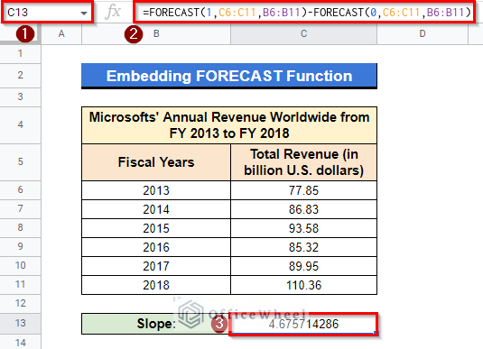
Formula Breakdown
- FORECAST(1,C6:C11,B6:B11)
This formula works similarly to the previous TREND function. Calculates the value of m+c for the given x & y data.
- FORECAST(1,C6:C11,B6:B11)-FORECAST(0,C6:C11,B6:B11)
However, returns the value of slope “m” after calculating “m+c-c”.
6. Combining FORECAST and INTERCEPT Functions
We can get the value of slope by using the combination of FORECAST and INTERCEPT functions also.
Steps:
- Select Cell C13, apply the following formula below, and press Enter-
=FORECAST(1,C6:C11,B6:B11)-INTERCEPT(C6:C11,B6:B11)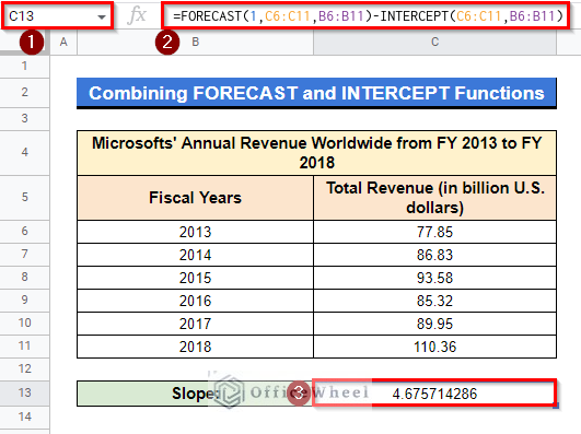
Formula Breakdown
- FORECAST(1,C6:C11,B6:B11)
The FORECAST formula here returns the value of m+c.
- INTERCEPT(C6:C11,B6:B11)
The INTERCEPT function here returns the value of the Y-axis intercept “c” only.
- FORECAST(1,C6:C11,B6:B11)-INTERCEPT(C6:C11,B6:B11)
Returns “m+c-c” which is basically equal to “m” which is the value of the slope.
Read More: How to Find P-Value in Google Sheets (With Quick Steps)
Similar Readings
- How to Search in Google Spreadsheet (5 Easy Ways)
- Find Uncertainty of Slope in Google Sheets (3 Quick Steps)
- How to Find Correlation Coefficient in Google Sheets
- Replace Space with Dash in Google Sheets (2 Ways)
7. Using Least Squares Method
The Least Squares formula to find the slope is as follows-
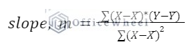
We will use a bunch of formulas such as AVERAGE, SUM functions, and some basic math.
To use this formula, we will need the dataset as shown below-
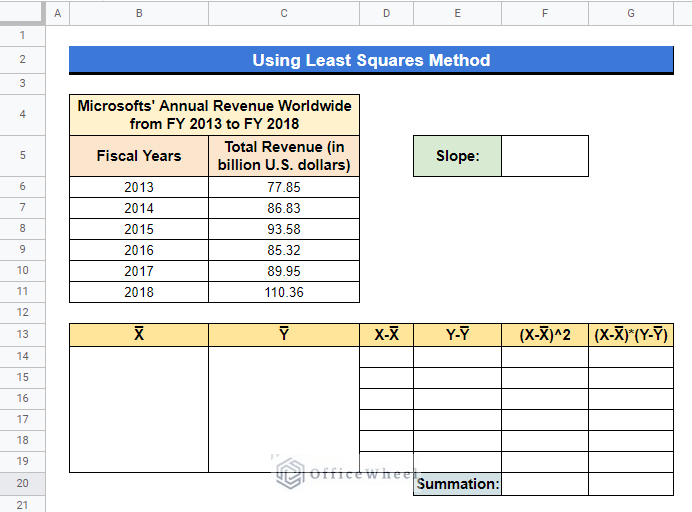
Steps:
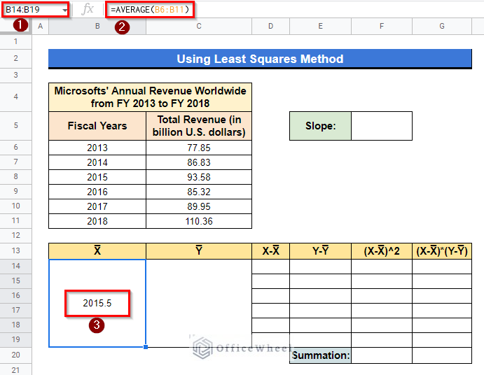
- First, select the merged cell B14:B19 then apply the following formula and press Enter–
=AVERAGE(B6:B11)Here, the formula will calculate the average value for all the values of independent variable X and will return the output as shown.
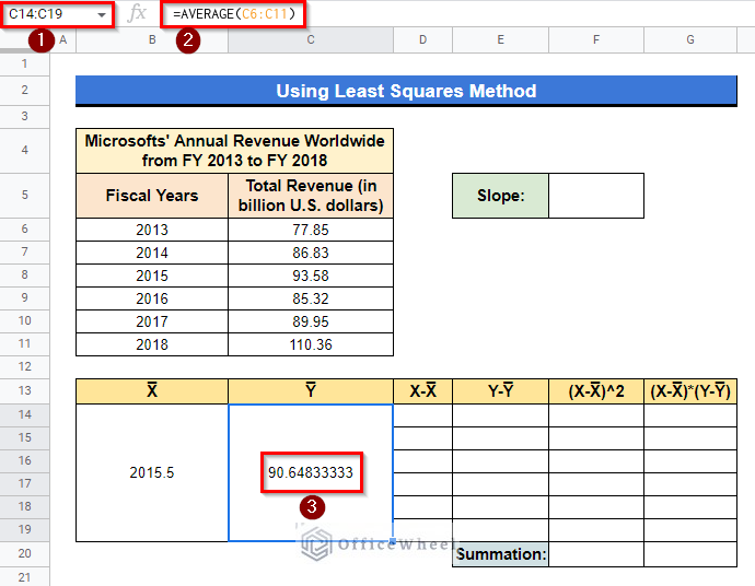
- Now, select merged cell C14:C19 and apply the following formula like previously.
=AVERAGE(C6:C11)Applying this formula will return the average of all values of dependent variable Y.
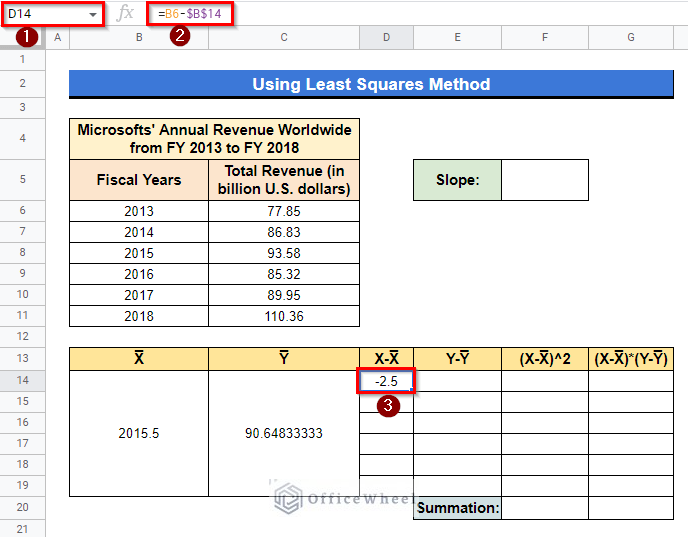
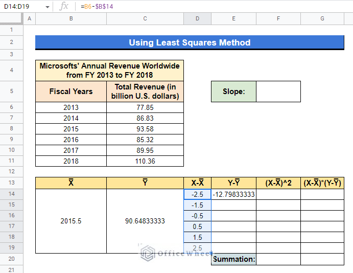
- After that, choose Cell D14, then input the following formula and press Enter–
=B6-$B$14This will calculate the difference between the value of X in Cell B6 and the average value of X that is X̅.
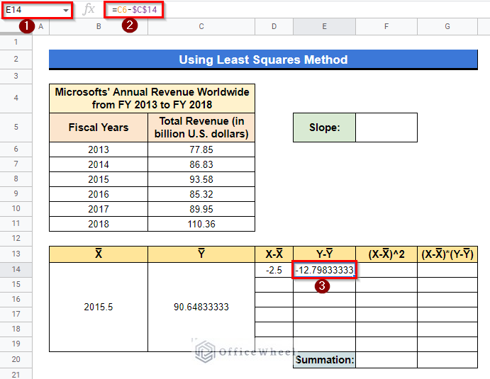
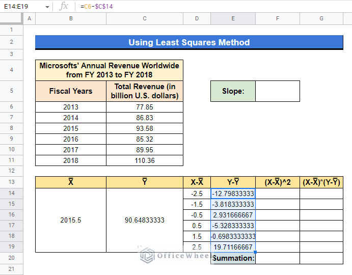
- Later, select Cell E14 and apply the following formula.
=C6-$C$14This formula will measure the difference between the value of Y in Cell C6 and the average value of Y that is Y̅.
- Now, select Cell D14 and drag down using the Fill handle icon as shown in the circled portion below.
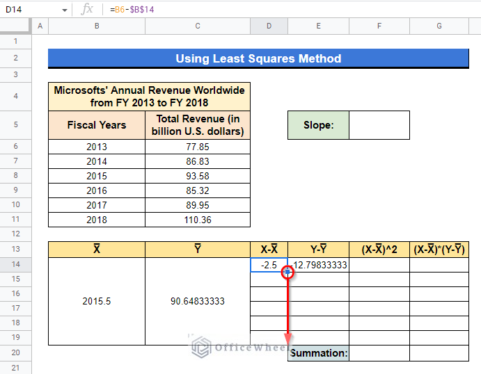
- Performing this, the formula will return the difference between X̅ and the rest of the other X values as well.
- Now, do the exact same by selecting Cell E14 and the result will be as follows.
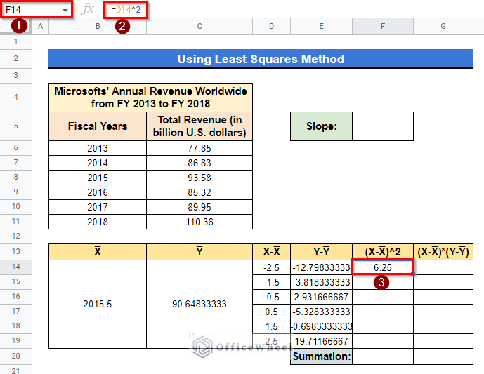
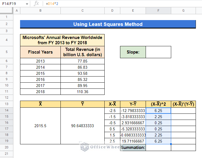
- At this point, we have to calculate the square value of (X-X̅) that is (X-X̅)2.
- Select Cell F14 and apply the following formula-
=D14^2- Positively it will calculate the square of (X-X̅) value which is in Cell D14. You can see the output in Cell F14.
- Drag down using the Fill handle icon as shown in the circled portion to get the square value of other (X-X̅) values as well.
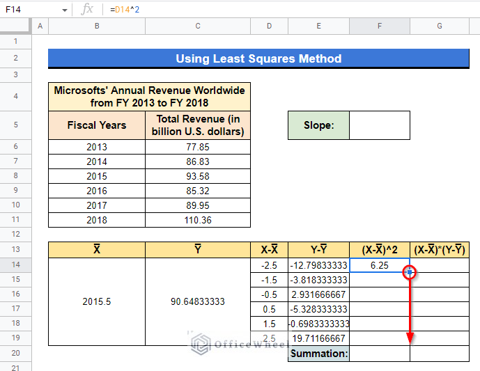
- This will calculate the square value of other (X-X̅) values.
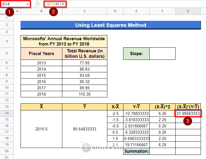
- Now, we have to calculate the product of (X-X̅) and (Y-Y̅) for each value of (X-X̅) and (Y-Y̅). Select Cell G14 and apply the following formula.
=D14*E14- Here, Cell D14 refers to the value of (X-X̅) and Cell E14 refers to the value of (Y-Y̅).
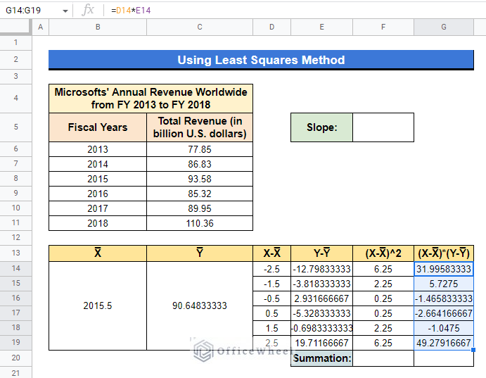
- Drag down using the Fill Handle icon in Cell G14 like previously and the result will be as follows.
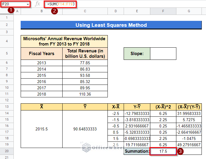
- Thereafter, select Cell F20 and apply the below formula.
=SUM(F14:F19)- Have a look at the Least Squares formula again. The formula requires the value of ∑(X-X̅)2. Consequently, the SUM function will calculate the sum of all the values of (X-X̅)2.
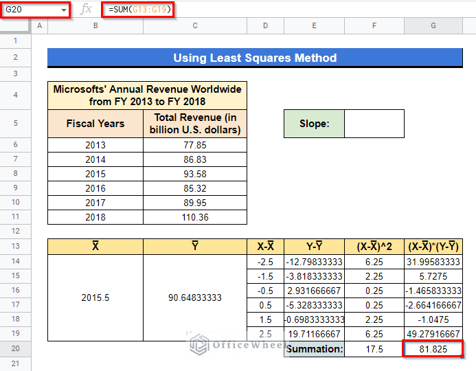
- Afterward, select Cell G20, apply the given formula below and press Enter–
=SUM(G14:G19)- The Least Squares formula requires the value of ∑(X-X̅)*(Y-Y̅).
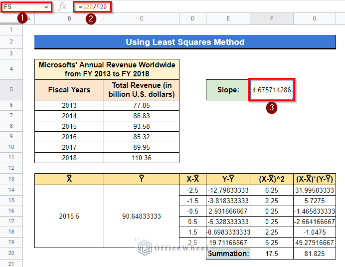
- Finally, select Cell F5 and apply the following formula below then press Enter–
=G20/F20- This formula is basically the representation of the Least Squares formula:
![]()
Here, Cell G20 refers to the value ∑(X-X̅)*(Y-Y̅) (the numerator of the Least Squares formula).
And Cell F20 refers to the value ∑(X-X̅)2 (the denominator of the Least Squares formula).
- Therefore, the value of the slope will return as the output in Cell F5 as shown below.
Read More: How to Find Merged Cells in Google Sheets (3 Ways)
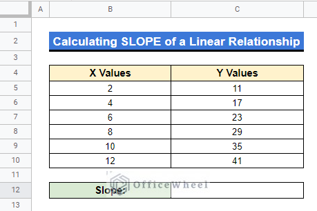
8. Calculating SLOPE of a Linear Relationship
You can apply any of the above methods to get the slope of a linear relationship but now we will solve this using the basic formula of slope. First, let me explain the formula.
Suppose, if there are any two points (x1,y1) and (x2,y2) on the straight line y=mx+c, then the value of slope “m” will be (y2-y1)/(x2-x1).
Now, if you have a dataset containing values of dependent variable y and independent variable x and if there is a linear relationship between them, we can use the above formula of slope to calculate the value of slope manually.
Suppose, in the below spreadsheet, Cell range B5:B10 contains values of independent variable X and Cell range C5:C10 contains values of dependent variable Y. And there is also a linear relationship between them.
Steps:
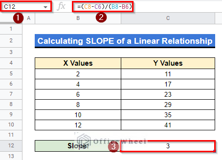
- Select Cell C12 and apply the following formula then press Enter–
=(C8-C6)/(B8-B6)- As I have said previously, (x1,y1) and (x2,y2) can be any two points on the linear line. Here, (x1,y1) indicates (Cell B6, Cell C6) and (x2,y2) refers to (Cell B8, Cell C8).
- The output will be shown in Cell C12 as follows.
Read More: How to Find Linear Regression in Google Sheets (3 Methods)
Conclusion
All the easiest and quickest ways to find the slope of graph in Google Sheets are described in this article. Hope this will definitely help with your work. Visit officewheel.com to explore more relevant articles.
Related Articles
- How to Find Hidden Rows in Google Sheets (2 Simple Ways)
- Find Uncertainty of Slope in Google Sheets (3 Quick Steps)
- How to Find Median in Google Sheets (2 Easy Ways)
- Find Frequency in Google Sheets (2 Easy Methods)
- How to Find Edit History in Google Sheets (4 Simple Ways)
- Find Largest Value in Column in Google Sheets (7 Ways)
- How to Find Trash in Google Sheets (with Quick Steps)