Merged cells become an obstacle often while performing various functions like if there is any merged cell in a range of cells, you can’t add any filter option in that range of cells. So, it is important to identify those and unmerge them in order to perform those functions. In this article, we have demonstrated 3 easy methods to find merged cells in Google Sheets.
A Sample of Practice Spreadsheet
Here is the spreadsheet used for explaining the methods. You can easily download it from here.
3 Easy Methods to Find Merged Cells in Google Sheets
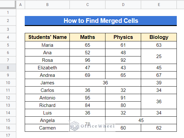
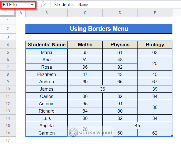
We will use the following sample dataset to demonstrate these methods accurately. The dataset represents some students’ grades in Maths, Physics and Chemistry subjects. Have a look, it contains some merged cells.
1. Combining ARRAYFORMULA and IF Functions
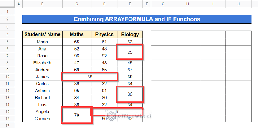
One of the best ways to find merged cells is to use the combination of the ARRAYFORMULA and IF functions in Google Sheets. The ARRAYFORMULA function commands with a single formula to each cell in the predefined data range. Within a range of cells, the IF function works based on a given logical expression and returns a given value if the logical expression is TRUE and returns another given value of the logical expression false. You can see that there are several merged cells in the following dataset.
Steps:
- In the following dataset, apply the following formula below in Cell G4 and press Enter–
=ARRAYFORMULA(IF(B4:E16="",ADDRESS(ROW(B4:E16),COLUMN(B4:E16)),))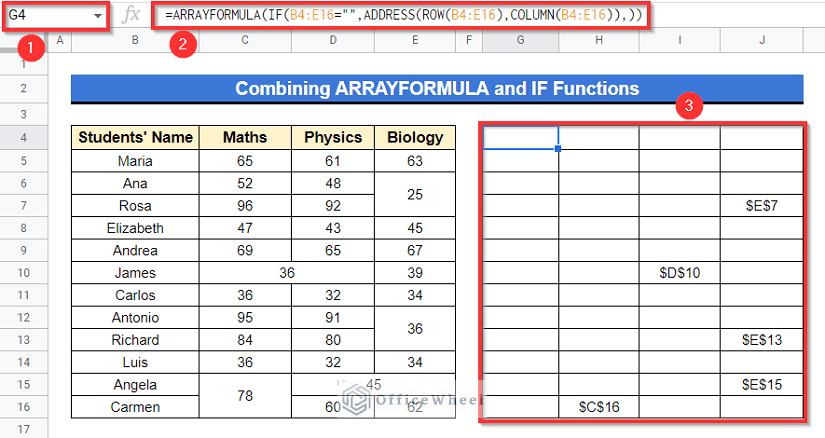
Formula Breakdown
- ADDRESS(ROW(B4:E16),COLUMN(B4:E16))
First, the ADDRESS function will return the cell references for every cell of the range.
- IF(B4:E16=””,ADDRESS(ROW(B4:E16),COLUMN(B4:E16)),)
Later, the IF function will perform logical test, if it gets any empty cell in merged cells then it will return the cell address otherwise will return blanks.
- ARRAYFORMULA(IF(B4:E16=””,ADDRESS(ROW(B4:E16),COLUMN(B4:E16)),))
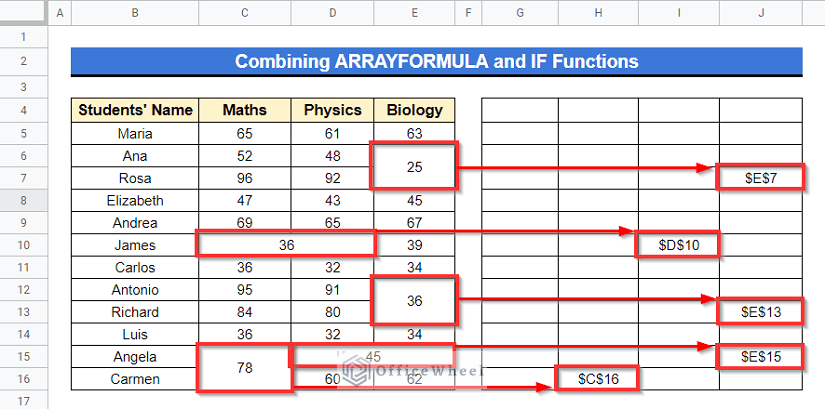
Finally, it will return the output for the range as an array in the table.
- After applying the formula, the merged cell references will appear and then you can easily identify those merged cells.
Read More: How to Find the Range in Google Sheets (with Quick Steps)
2. Using Borders Menu
We can simply detect merged cells visually by applying a bold border style over the whole range of cells. When you have a large dataset, it will easily highlight the merged cells with thick borders.
Steps:
- First of all, select the Cell range B4:E16.
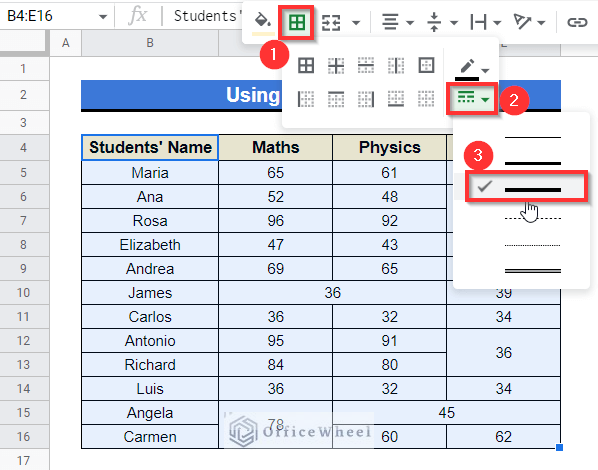
- Next at the toolbar, select the Border ribbon, then go to the Border style menu and apply the Bold Border Style.
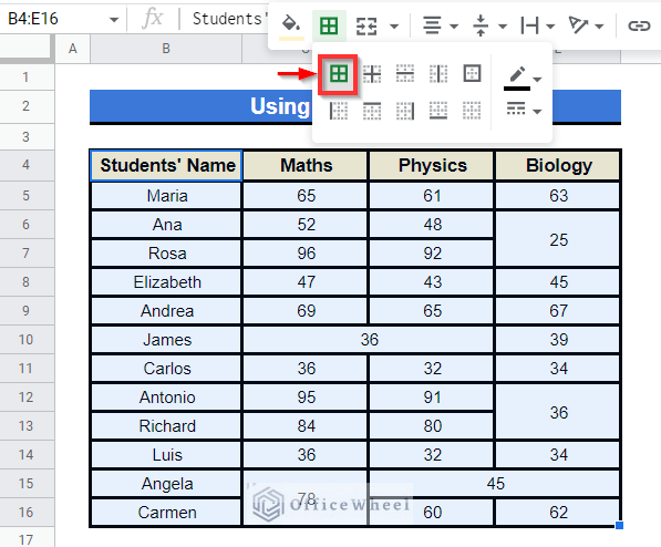
- Thereafter, click on the All borders option in the Borders.
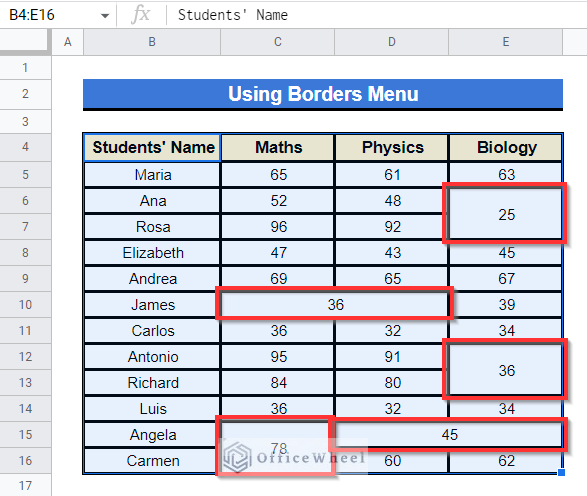
- Finally, those merged cells are unraveled now and you can count those visually by yourself.
Read More: Find Value in a Range in Google Sheets (3 Easy Ways)
Similar Readings
- How to Find Edit History in Google Sheets (4 Simple Ways)
- Find Quartiles in Google Sheets (4 Useful Methods)
- How to Find and Delete in Google Sheets (An Easy Guide)
- Use FIND Function in Google Sheets (5 Useful Examples)
- How to Find Largest Value in Column in Google Sheets (7 Ways)
3. Applying Conditional Formatting Option
The use of Conditional Formatting option in Google Sheets can aid in clarifying the shapes or patterns of a range of cells in your dataset. For example, you can change the background color shading of cells or change the font types into different cells using the conditional formatting option. In brief, this setting can help to present your dataset enchantingly.
3.1 For Merged Cells Along Rows
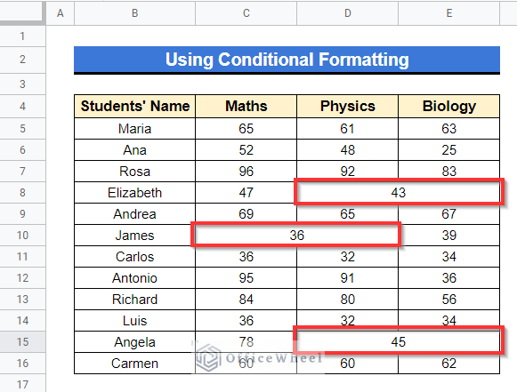
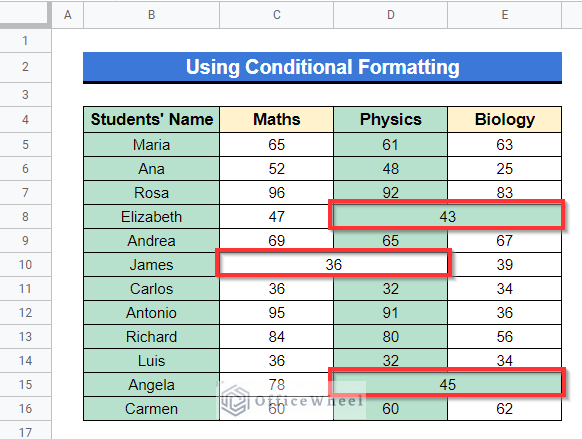
In the following dataset below, we can see that some cells are merged mistakenly along some rows. Our goal is to make them visually clarified to count.
Steps:
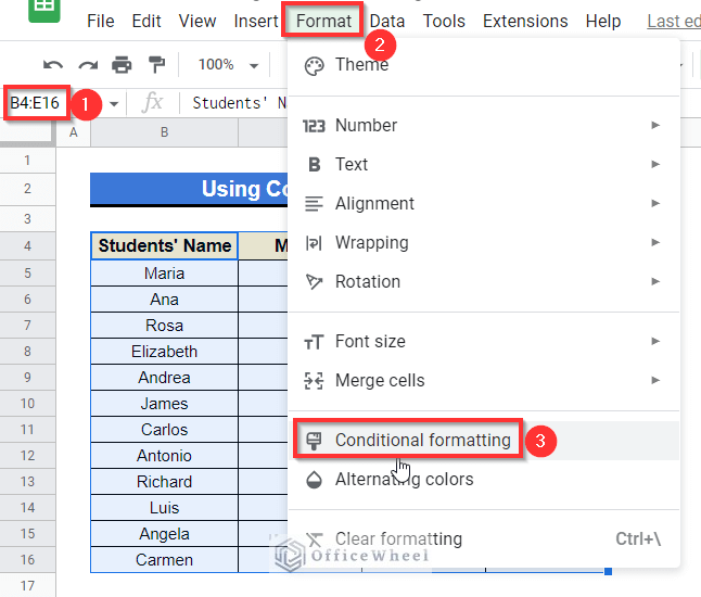
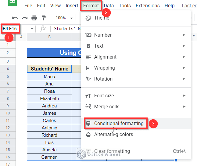
- Select the Cell range B4:E16 and then go to the Format menu at the toolbar, after that click on the Conditional formatting.
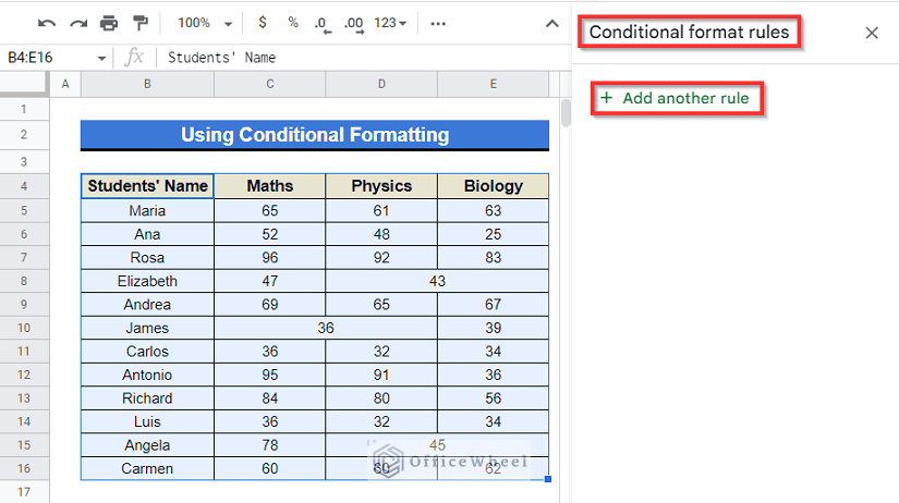
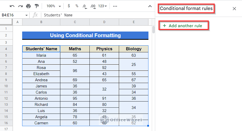
- A sidebar will appear to the right of your spreadsheet titled “Conditional format rules”. There, select the “Add another rule” option.
- Thereafter, you will find the Find cells if Drop-down Select the “Custom formula is” option from that drop-down menu.
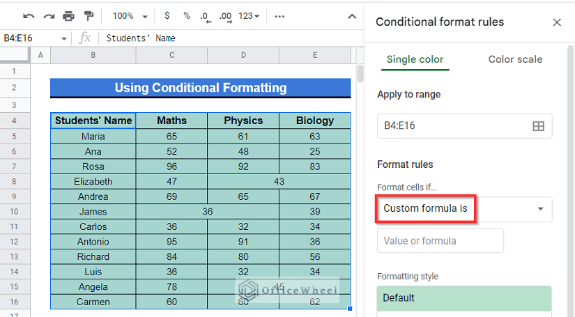
- Next, apply the formula below in the “Value or formula” bar and click on Done.
=MOD(COLUMN(),2)=0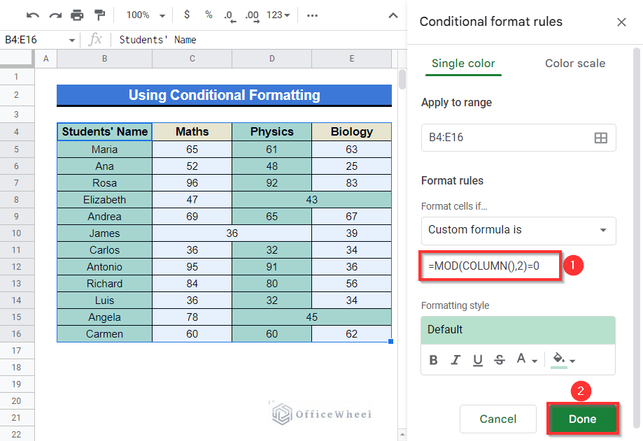
Formula Breakdown
- COLUMN()
Returns the column number of the specific cell.
- MOD(COLUMN(),2)=0
The MOD function will then divide the column number by 2, if it returns to zero then the cell will be formatted with the formatting color. So, actually, this will highlight every even column starting from the first column of the range. The merged cells contain the reference of the first cell of them, so for merged cells, the color pattern will break and that will help us to identify them.
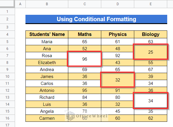
- You can identify some color pattern intercepted cells visually and easily because those are merged.
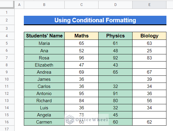
- If there were no merged cells, the color pattern would be as follows after applying the formula shown previously.
Read More: Find All Cells With Value in Google Sheets (An Easy Guide)
3.2 For Merged Cells Along Columns
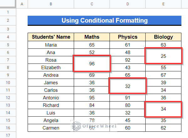
In another case, there are some merged cells along some columns in the below spreadsheet you can see. We will mark out those merged cells like previously.
Steps:
- Choose Cell range B4:E16, go to the Format menu at the toolbar and then select the “Conditional formatting” option like previously.
- Sidebar titled “Conditional format rules” will appear, select “Add another rule”.
- Apply the following formula in the “Value or formula” bar after selecting the “Custom formula is” option from the “Formula cells if” Drop-down menu, select the Fill color as you wish and then press on “Done”.
=MOD(ROW(),2)=0
Formula Breakdown
- ROW()
It will return the row number of the specific cell.
- MOD(ROW(),2)=0
Later, the MOD function will then divide the row number by 2, if it returns to zero then the cell will be formatted with the formatting color. Basically, it will highlight every even row starting from the first row of the range. The merged cells use the reference of the first cell of them, that’s why the color pattern will change and that will help us to identify them.
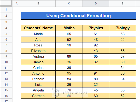
- Finally, you will be able to mark out those merged cells by identifying the color intercepted zones simply.
- If there were no merged cells in that dataset, the color pattern would be as follows in that range of cells after applying that formula.
Read More: How to Use Find and Replace in Column in Google Sheets
Conclusion
As I have said, merged cells are a barrier in the way of performing several operations. But if there is any of them, it is much easier to identify those and unmerge them. In this article, we have tried to illustrate 3 easy ways to find merged cells in Google Sheets. Hope this will help you with your task. Visit officewheel.com to explore more relevant articles.
Related Articles
- How to Find P-Value in Google Sheets (With Quick Steps)
- Find Slope of Trendline in Google Sheets (4 Simple Ways)
- How to Find Median in Google Sheets (2 Easy Ways)
- Find Uncertainty of Slope in Google Sheets (3 Quick Steps)
- How to Find Linear Regression in Google Sheets (3 Methods)
- Find Slope of Graph in Google Sheets (With Easy Steps)
- How to Find Correlation Coefficient in Google Sheets