How to Find Correlation Coefficient in Google Sheets

A correlation coefficient is a metric that expresses a correlation, or a statistical link between two variables, in numerical terms. In brief, correlation coefficient is important to understand the significance and direction of the linear correlations between pairs of variables. In this article, we have demonstrated 5 easy ways to find correlation coefficient in Google Sheets.

Table of Contents

A Sample of Practice Spreadsheet

You can download the spreadsheet used for describing methods for this article from here.

Find Correlation Coefficient

What Is Correlation Coefficient ?

The correlation coefficient indicates how closely two variables are related. There are three different types of data correlation: Positive correlation, Negative correlation, and No correlation.

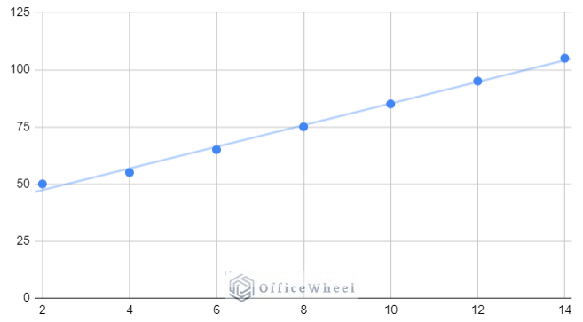
According to the Positive correlation coefficient, when one variable rises, another variable rises as well. A positive correlation coefficient has a value larger than 0.

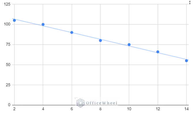
According to the Negative correlation coefficient, as one variable rises, another variable falls. The negative correlation coefficient has a value that is less than 0.

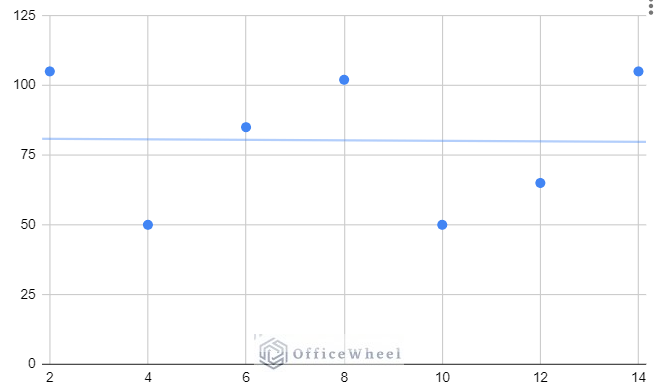
The correlation coefficient, whose value is near to or equal to 0, indicates that there is no association between two variables.

5 Easy Methods to Find Correlation Coefficient in Google Sheets

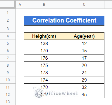
We will be using the following dataset to demonstrate methods in this article. The dataset represents some persons’ height and age.

1. Using CORREL Function

The built-in CORREL function in Google Sheets returns the value of the correlation coefficient of two ranges of cells. The first one is the cell ranges of Y data which is the dependent variable. The second range of cells is the data of independent variable X.

1.1 Inserting Data Manually

We can simply use this CORREL function by typing down the data of both variables within the formula. It’s not a feasible method for a long dataset but maybe helpful for split values.

Steps:

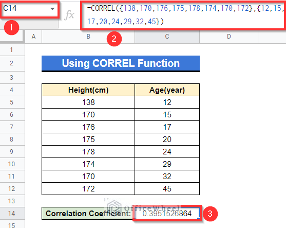
In the following dataset, select Cell C14 and type the following formula then press Enter-

=CORREL({138,170,176,175,178,174,170,172},{12,15,17,20,24,29,32,45})

Here, the data in the first {} are the values of dependent variable Y and the data in the second {} are the values of independent variable X.

1.2 Using Cell References

We can simply use cell references within the CORREL formula to get the correlation coefficient.

Steps:

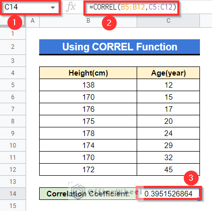
In Cell C14, apply the following formula and then Enter–

=CORREL(B5:B12,C5:C12)

Here, Cell range B5:B12 indicates the dependent variables’ values while Cell range C5:C12 represents the independent variables’ values.

2. Combining RSQ and SQRT Functions

Correlation coefficient is the square root of coefficient of determination. Here, we will first calculate the value of the coefficient of determination using the RSQ function. Then we will get the result of the square root of that as correlation coefficient using the SQRT function.

Steps:

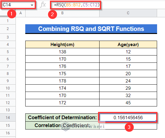
First, select the Cell C14 in the following dataset and enter the following formula-

=RSQ(B5:B12,C5:C12)

This will calculate the value of the coefficient of determination.

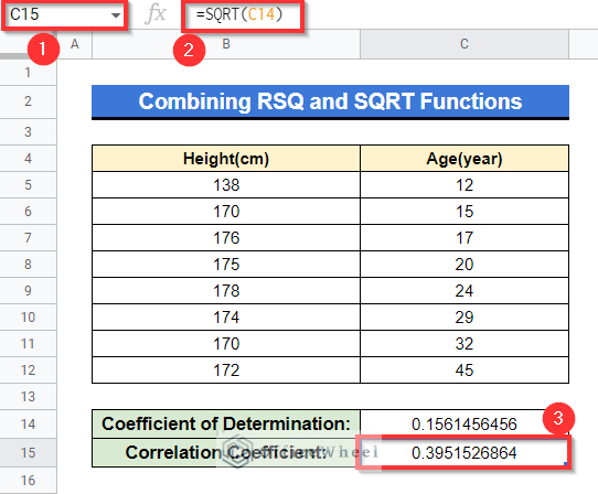
Now, activate Cell C15, put the following formula below there and press Enter–

=SQRT(C14)

In the formula, Cell C14 refers to the cell that carries the value of the coefficient of determination.

3. Applying PEARSON Function

The formula of PEARSON is as follows-

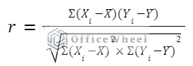
Great news is, Google Sheets has a built-in PEARSON function for this formula. The Pearson correlation coefficient is returned by the PEARSON function after receiving two arrays as parameters in which the first one is for the dependent variable and the 2nd one is the values of the independent variable. We can easily find correlation coefficient in Google Sheets using this formula.

Steps:

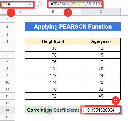
First, select Cell C14 and then apply the following formula and press Enter–

=PEARSON(B5:B12,C5:C12)

Then you will get the same output as before.

Similar Readings

4. Using PEARSON Formula Manually

If you got an assignment or an upcoming test based on correlation coefficient, I would prefer you to follow this method to understand your topic properly. Before this, I have already shown you the use of the PEARSON function. But now, we will learn how to solve the Pearson correlation coefficient manually in Google Sheets. The AVERAGE, SUM, and SQRT functions will come up in this manner.

The basic equation in this case is as follows:

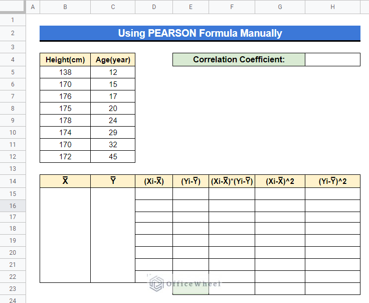
We will make a dataset for this as shown below-

Steps:

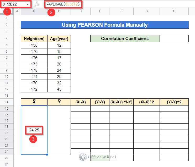
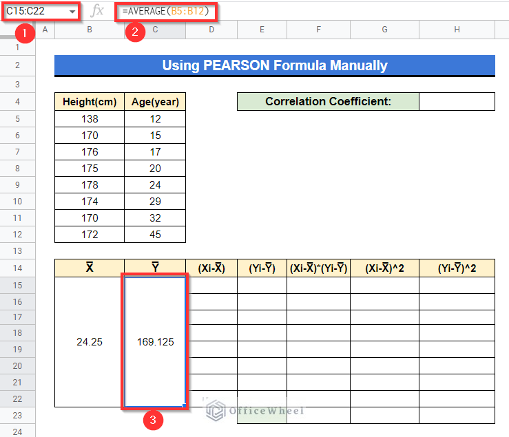
First of all, we have to find X̅ (average value of independent variable X) and Y̅ (average value of dependent variable Y). Select Merged Cell B15:B22, apply the following formula-

=AVERAGE(C5:C12)

Here, Cell range C5:C12 refers to the values of independent variable X.

Secondly, do the same for the Y variable as well. Select Merged cell C15:C22 and then apply the following formula-

=AVERAGE(B5:B12)

Cell range B5:B12 refers to the values of the Y variable. The formula here will calculate the average of Y values.

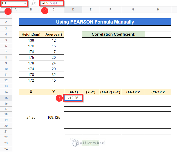
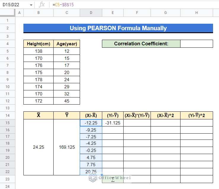
Now, we have to calculate the values of (X_i-X̅) and (Y_i-Y̅). For that, we will apply the following formula in Cell D15.

=C5-$B$15

This will calculate the difference between the value of X in Cell C5 and the average value of X that is X̅.

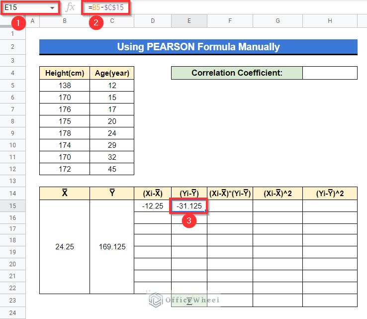
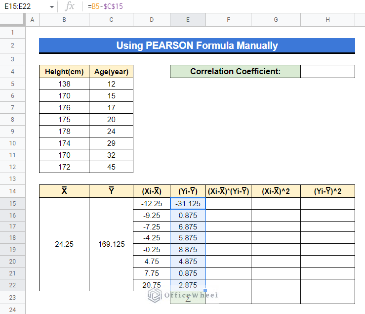
And then we will apply the below formula into Cell E15.

=B5-$C$15

This will measure the difference between the value of Y in Cell B5 and the average value of Y that is Y̅.

After that, select Cell D15 and then simply drag down using the Fill handle icon as shown in the circled portion below.

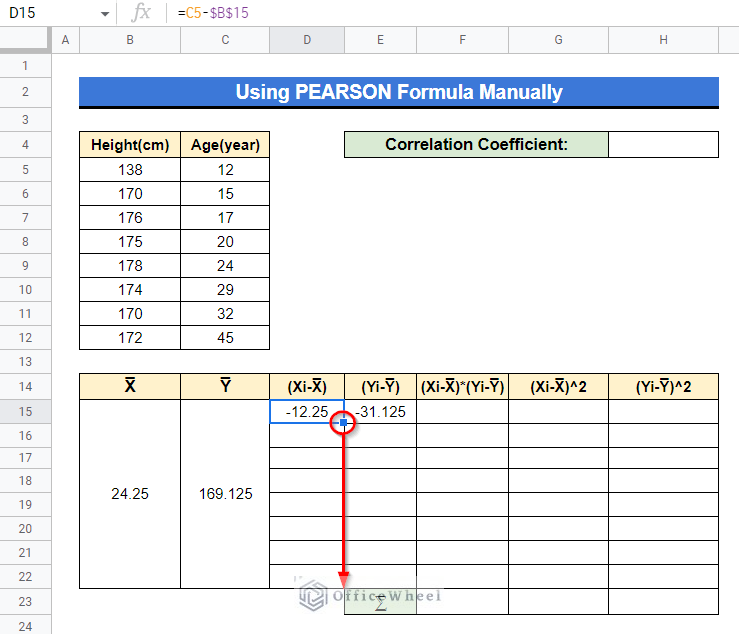
This will calculate the difference between X̅ and the rest of the other X values as well.

Now, do the exact same by selecting Cell E15 and the result will be as follows.

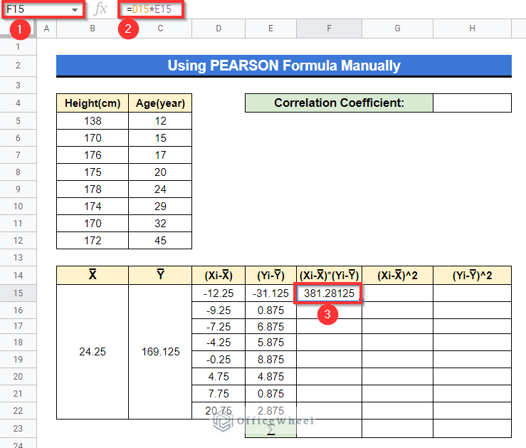
At this point, we have to calculate the product of (X_i-X̅) and (Y_i-Y̅) for each value of (X_i-X̅) and (Y_i-Y̅). Select Cell F15 and apply the following formula.

=D15*E15

Here, Cell D15 refers to the value of (X_i-X̅) and Cell E15 refers to the value of (Y_i-Y̅).

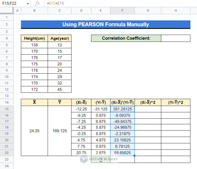
Drag down using the Fill Handle icon in Cell F15 like previously and the result will be as follows.

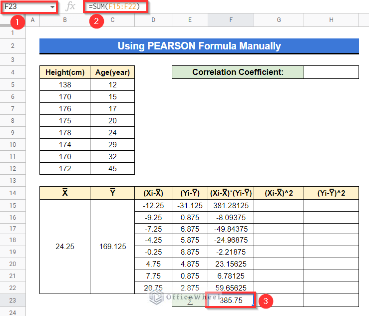
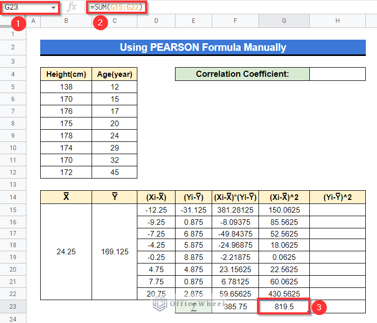
Select Cell F23 and apply the below formula. Have a look at the Pearson formula again. We need the value of ⅀(X_i-X̅)*(Y_i-Y̅).

=SUM(F15:F22)

The SUM function we calculate the summation of all the values of the product (X_i-X̅)*(Y_i-Y̅).

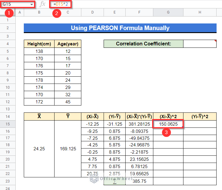
Next, we need to calculate the square values of all the (X_i-X̅) and (Y_i-Y̅) Apply the formula into the box below in Cell G15 and press Enter–

=D15^2

Obviously it will calculate the square of (X_i-X̅) value which in Cell D15. You can see the output in Cell G15.

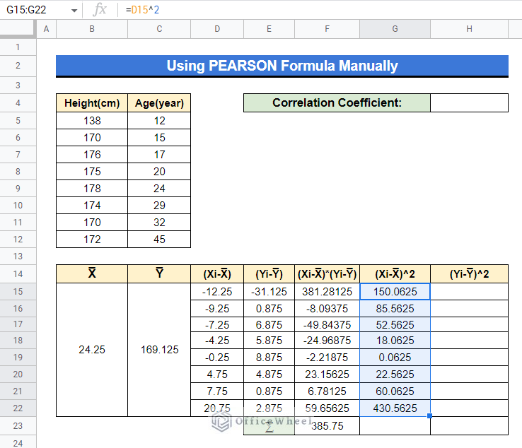
Drag down using the Fill handle icon as shown in the circled portion to get the square value of other (X_i-X̅) values as well.

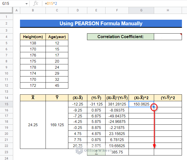
After that the square value of other (X_i-X̅) values.

Thereafter, choose Cell G23 and apply the following formula below.

=SUM(G15:G22)

Going through this, the summation of all (X_i-X̅)² values across the Cell range G15:G22.

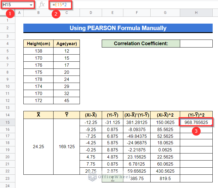
Next, select Cell H15, apply the following formula below and press Enter–

=E15^2

This will determine the square of (Y_i-Y̅) value which is in Cell E15. The output will be as follows in Cell H15.

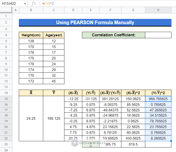
Now drag down using the Fill handle icon in Cell H15 like previously to get the square of other (Y_i-Y̅) values as well.

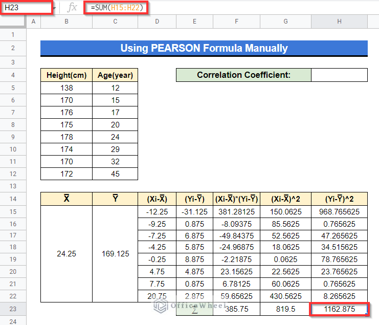
After that, activate Cell H23, give input the following formula and press Enter–

=SUM(H15:H22)

Here, the SUM function will calculate the summation of all the (Y_i-Y̅)² values across Cell range H15:H22.

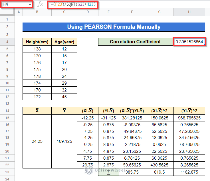
Finally, select Cell H4 and apply the following formula below then press Enter–

=(F23)/SQRT(G23*H23)

This formula is basically the representation of the Pearson formula: 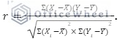Here, Cell F23 refers to the value ⅀(Xi-X̅)(Yi-Y̅) (the numerator of the Pearson formula).

SQRT(G23*H23) refers to the value of √(⅀(Xi-X̅)^2*(Yi-Y̅)^2) (the denominator of the Pearson formula).

Therefore, the value of the correlation coefficient will be as follows in Cell H4.

5. Using Chart Feature

We can create a chart and get the value of the coefficient of determination from that. Then, calculating the square root value from that, we will simply get the value of the correlation coefficient.

Steps:

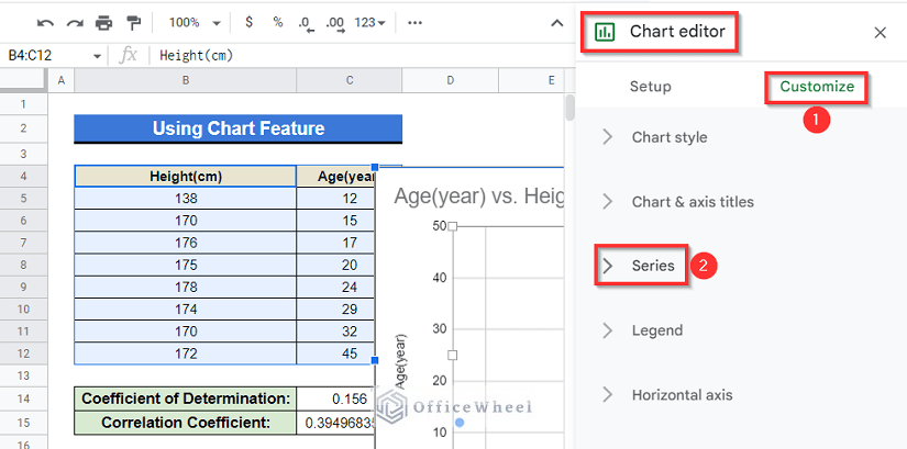
Select the Cell range B4:C12, click on the Insert chart ribbon from the toolbar at top.

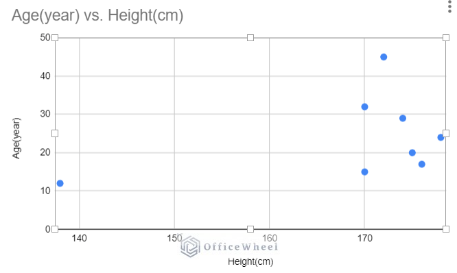
A scattered chart will appear on your screen.

Now, from the sidebar titled “Chart editor”, go to the Customize menu then select “Series” drop-down.

Afterward, in that drop-down menu, mark the Trendline box and then mark the Show R²

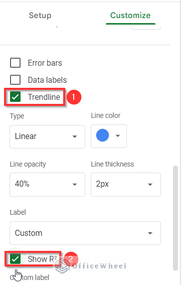
Following this, you will see that the value of coefficient of determination that is R² will appear on your chart.

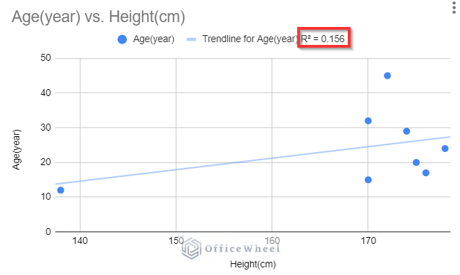
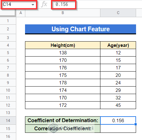
Therefore, type down this value “0.156” into Cell C14 in the following dataset.

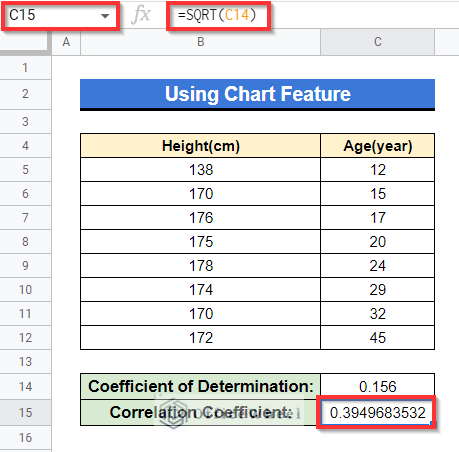
Finally, apply the following formula into Cell C15 and press Enter–

=SQRT(C14)

In the formula, Cell C15 refers to the cell that carries the value of coefficient of determination.

The output showing in Cell C15 is the value of correlation coefficient.

Conclusion

The article contains 5 efficient methods to find correlation coefficient in Google Sheets. Hope this will help with your task. Visit officewheel.com to explore more relevant articles.

How to Find Correlation Coefficient in Google Sheets

A Sample of Practice Spreadsheet

What Is Correlation Coefficient ?

5 Easy Methods to Find Correlation Coefficient in Google Sheets

1. Using CORREL Function

1.1 Inserting Data Manually

1.2 Using Cell References

2. Combining RSQ and SQRT Functions

3. Applying PEARSON Function

4. Using PEARSON Formula Manually

5. Using Chart Feature

Conclusion

Related Articles

Adrey

Leave a reply Cancel reply