Google Sheets is an application powerful enough to recognize most values and patterns in its spreadsheets, making it that much easier to search for user-specific values in it. In this article, we will take advantage of this capability to see all the ways we can use to find and delete in Google Sheets.
Let’s get started.
How to Find and Delete in Google Sheets
1. Find and Delete Specific Value in Google Sheets
The Simplest Way: Using the Find and Replace Feature
Find and Replace is the most standard option available that we can use to find a value in Google Sheets. While the name is Find and “Replace”, we can always replace our searched value for an empty space to treat it as deleted.
To open the Find and Replace window, use the keyboard shortcut CTRL+H (CMD+H for Mac) or navigate to the feature from the Edit tab.
Here in the window, search for your desired value. We have chosen the name “Rachel” from our dataset of names.
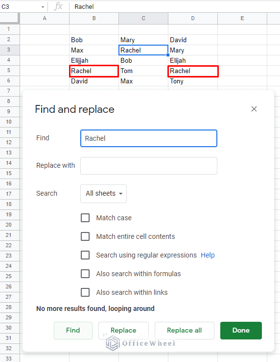
Note: Clicking on Find will cycle through all the instances of the searched word. It is always good to check beforehand for matching values.
To delete the searched value, simply leave the Replace with field empty. As for other conditions, change as necessary. We have confined our find and delete process to the current worksheet (This sheet).
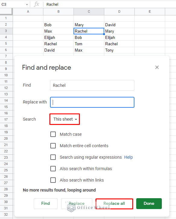
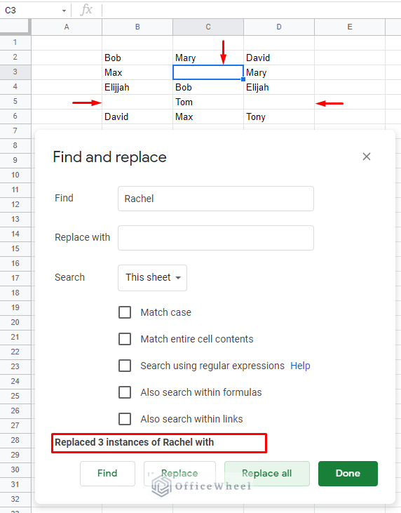
Click Replace all to find and delete the searched value in Google Sheets.
Find and Delete Multiple Values with Partial Match using Regular Expression
We can search for multiple values in Find and Replace by taking advantage of the fact that some words share the same characters in similar positions. We do this by using regular expressions.
Regular expressions are a special sequence of characters that help us fine-tune sour searches in Google Sheets.
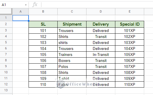
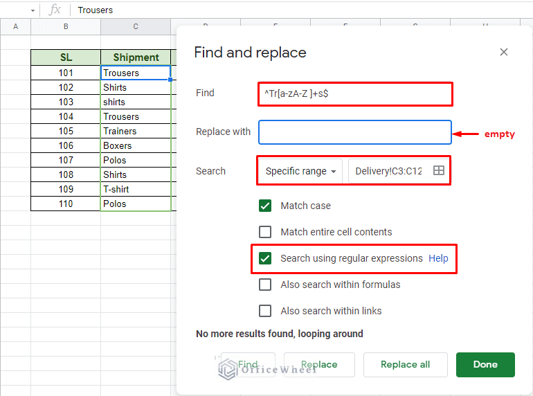
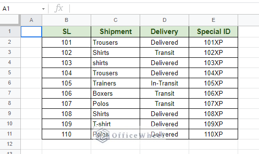
For example, we want to find and delete “Trousers” and “Trainers” from the following worksheet.
Lucky for us, both words start with ‘Tr’ and end with an ‘s’. Our regular expression will be:
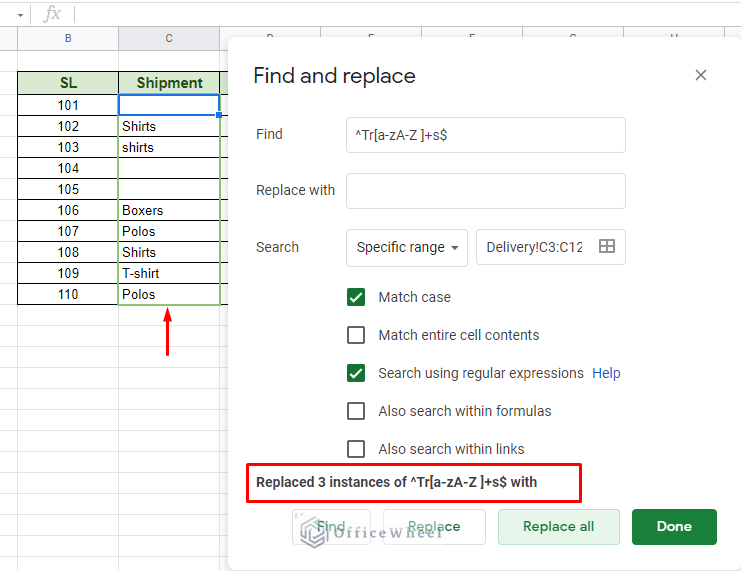
^Tr[a-zA-Z ]+s$Setting up our conditions in the Find and Replace window:
Just like before, click Replace all to find and delete all searched values:
Read More: How to Use Find and Replace in Column in Google Sheets
Removing Specific Symbols or Value within a Cell with Function
So far, we have seen how to find and delete entire values from cells in Google Sheets. This time, we will see how to remove partial values from cells and present them in a different range. Of course, the best way to do this is with functions, and we have two functions in mind for slightly different scenarios.
Note that these functions follow the same deleting idea, that is to replace the found value with no value (empty).
Using SUBSTITUTE Function to Remove Symbols
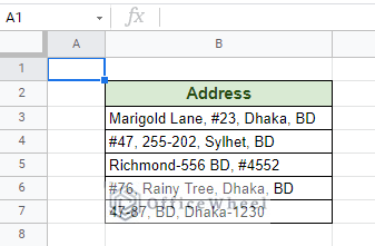
First up, we have the always reliable SUBSTITUTE function. We will use this function to specifically find and delete symbols in Google Sheets.
Our symbol of choice is the “#” from the following dataset:
Our formula:
=SUBSTITUTE(B3,"#","")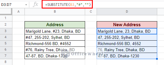
Quite easy, isn’t it?
Now, what if we want to delete multiple symbols in Google Sheets? Let’s say for both “#” and “-“.
SUBSTITUTE cannot take multiple values; however, we can go around this limitation by using one function inside another. Nested SUBSTITUTE functions if you will.
=SUBSTITUTE(SUBSTITUTE(B3,"#",""),"-","")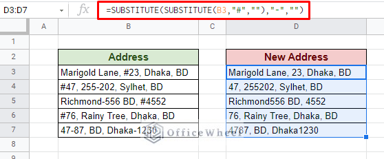
Read More: How to Remove Comma in Google Sheets (3 Easy Ways)
Using REGEXREPLACE to Find and Delete Text
On the other hand, finding and deleting text values from within a cell is not so easy. We once again must take the help of regular expressions which will be used in the REGEXREPLACE function.
REGEXREPLACE has similar workings to that of SUBSTITUTE, only this time, we are using regular expressions to find our value.
For this example, we will try and remove the text “BD” from our cells. Our formula:
=REGEXREPLACE(B3,"(.*)BD(.*)","$1 $2")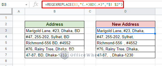
Formula Breakdown:
- B3: The cell reference to our string.
- “(.*)BD(.*)”: This is our regular expression to highlight the text “BD”. The “(.*)” before and after the text refers to any characters or strings that may be present in those positions around “BD”.
- “$1 $2”: This is our replacement argument. The $1 and $2 refer to the first and second “(.*)” of the regular expression. This means that this argument will replace the current string with whatever was before or after our removed text, “BD”.
Tip: You can combine the SUBSTITUTE and REGEXREPLACE functions to remove any commas from the result. You can even add TRIM for good measure to remove any extra whitespaces.
=TRIM(SUBSTITUTE(REGEXREPLACE(B3,"(.*)BD(.*)","$1 $2"),",",""))Read More: Use REGEXREPLACE to Replace Multiple Values in Google Sheets (An Easy Guide)
Similar Readings
- How to Search in Google Spreadsheet (5 Easy Ways)
- Find Uncertainty of Slope in Google Sheets (3 Quick Steps)
- How to Find Correlation Coefficient in Google Sheets
- Use FIND Function in Google Sheets (5 Useful Examples)
- How to Find Slope of Trendline in Google Sheets (4 Simple Ways)
2. Find and Delete Row Containing Value in Google Sheets
Using a Data Filter
Data Filters are a great approach to finding rows of data over a large spreadsheet. This also means that we can utilize it to delete rows of data as well. Let’s see how we can achieve it step by step.
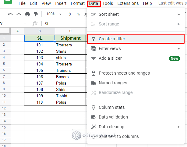
Step 1: Apply the Data Filter. Select any cell in the dataset and navigate to the Data tab then select Create a filter.
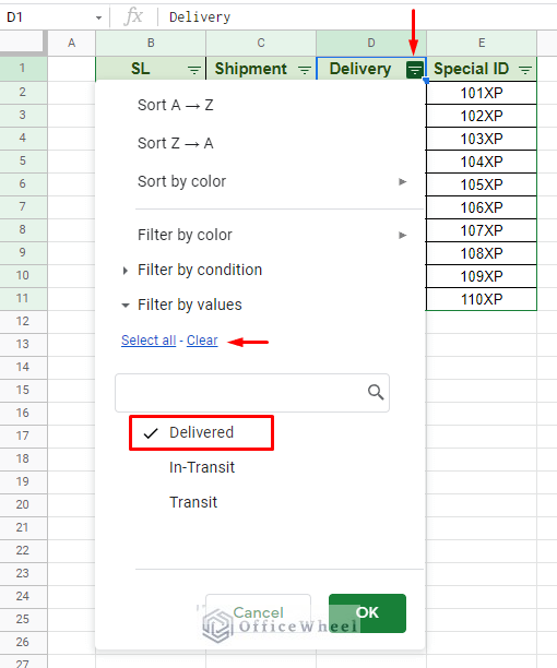
Step 2: With the filter created, we will look to delete all rows that have the Delivery status as Delivered. Click on the drop-down icon. First, select the Clear option to remove any selections. Then select Delivered.
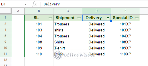
Step 3: Clicking OK will present you with all the entries that have the status Delivered.
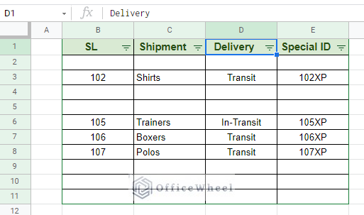
Step 4: Now, simply deleting these values will not be enough as it will leave blank rows when the table is unfiltered again. As we see here:
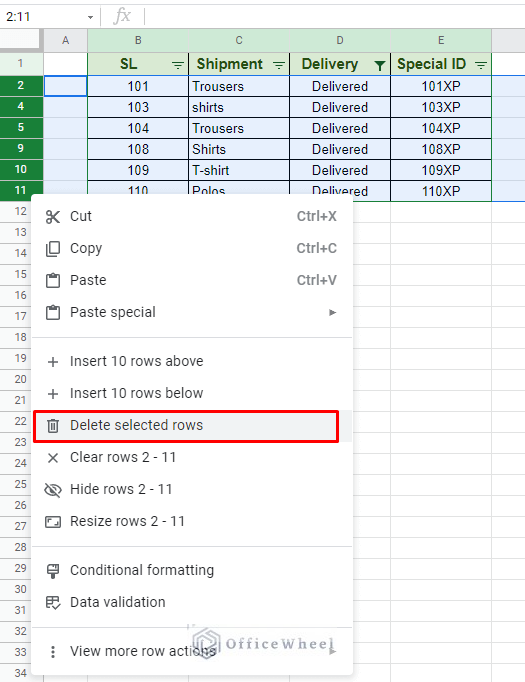
No, what we have to do is delete the rows entirely. We do this by selecting the row headers, right-click to bring up the options, and finally, select Delete selected rows.
Our result after un-filtering the dataset:
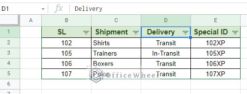
We have successfully found and deleted entire rows of data using the Data Filter.
Read More: How to Find Hidden Rows in Google Sheets (2 Simple Ways)
Using FILTER Function to Match and Delete Rows
If we are crafty enough, or just are aware of the capabilities of Google Sheets, we will know that any form of match, reference, or filter is possible here.
In this section, we will look specifically at how we can find and remove data according to a reference in another cell.
We have the following worksheet:
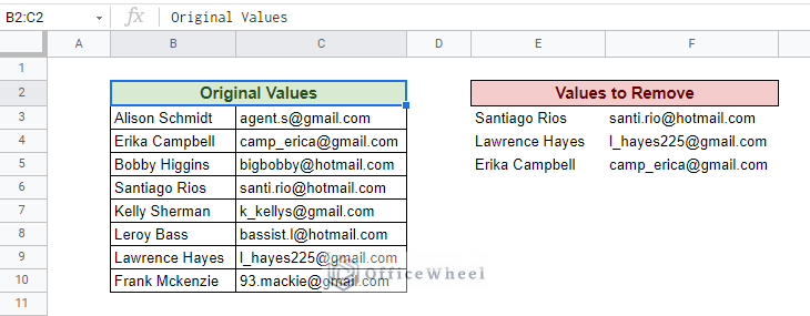
From the Original Values table, we want to remove the entries given in the Values to Remove table and present them in a separate dataset.
The formula we use is a combination:
=FILTER($B$3:$C$10,ISERROR(MATCH(B3:B10&C3:C10,E3:E&F3:F,0)))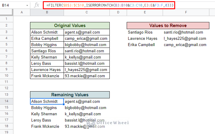
Formula Breakdown
- MATCH(B3:B10&C3:C10,E3:E&F3:F,0): There’s nothing complicated about the MATCH function. The only thing to note here is that we have combined the two columns from both tables so that both columns match. If you have multiple columns to match, simply add them on with an ampersand (&).
- ISERROR: This function acts as our logical condition. If a match does not occur, this function will return TRUE. It enables the FILTER function to return unmatched values only.
- $B$3:$C$10: The range of our table from which our values will be matched or extracted.
Note: We have also kept the range of the Values to Remove table open-ended, E3:E. This is to make the function slightly more dynamic as it will now consider any newly added values.
Read More: How to Remove Numbers from a String in Google Sheets
Using Google Apps Script
Oftentimes, especially in advanced cases, user requirements may not be satisfied with existing functions or their combinations. Such complicated needs can only be satisfied by creating a function that directly solves the problem. And what better way to do that than by using Google Apps Script.
Let’s say we want to automate the Data Filter method that we previously discussed. Deleting entries (entire rows) that have the status Delivered. We can perform this with a click of a button thanks to Apps Script.
To find this feature, navigate to the Extensions tab.
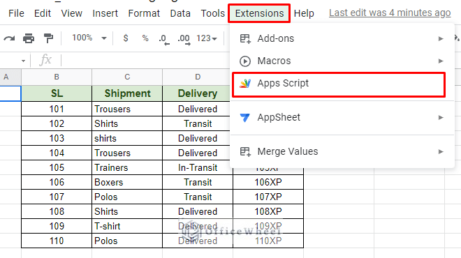
Here, type in the following script code:
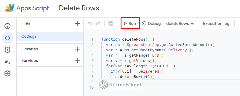
function deleteRows() {
  var ss = SpreadsheetApp.getActiveSpreadsheet();
  var s = ss.getSheetByName('Delivery');
  var r = s.getRange('D:D');
  var v = r.getValues();
  for(var i=v.length-1;i>=0;i--)
    if(v[0,i]=='Delivered')
      s.deleteRow(i+1);
};
Save and click Run.
Code Breakdown:
- The ‘Delivery’ in line 3 defines the sheet name in the current active spreadsheet to target.
- The ‘D:D’ in line 4 defines the range or column where the match occurs.
- Our value to match is ‘Delivered’. You can find it in line 7 of the code.
All of the above values can be changed according to the user’s need, and it is highly recommended.
Our result:
Before applying Script
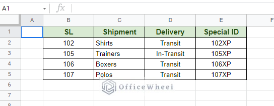
After applying Script
3. Find and Remove Whitespaces in Google Sheets
Sometimes, you may find entries or cell values that sport more than one space between the text. It can be because of a user error or, more commonly, if certain values were removed.
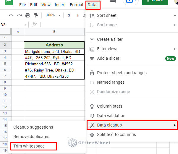
Thankfully, we have a built-in feature to eliminate these extra spaces in Google Sheets called Trim whitespaces.
You can access this feature from the Data tab.
Data > Data cleanup > Trim whitespaces
Alternatively, you can use the TRIM function to automatically find and delete whitespaces in Google Sheets:
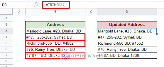
An advantage of the TRIM function is that you can use it with other text functions.
Final Words
That concludes all the different scenarios of find and delete in Google Sheets. As you have seen, Google Sheets can recognize more than just simple values, allowing us to work with all of them with ease. We hope that you’ve found our discussion fruitful.
Please feel free to leave any queries or advice you might have for us in the comments section below.
Related Articles for Reading
- How to Search in Google Spreadsheet (5 Easy Ways)
- Easy Guide to Replace Formula with Value in Google Sheets
- How to Find Trash in Google Sheets (with Quick Steps)
- Find Value in a Range in Google Sheets (3 Easy Ways)
- How to Find Edit History in Google Sheets (4 Simple Ways)
- Find All Cells With Value in Google Sheets (An Easy Guide)
- How to Find Median in Google Sheets (2 Easy Ways)
- Replace Space with Dash in Google Sheets (2 Ways)