One technique to examine a group of numbers and identify the core value is to calculate the AVERAGE. When a teacher takes a test on a group of students, for instance, he may determine how well the class performed overall by looking at the AVERAGE grade. And we all know that Google Sheets or Excel are the most used software in anywhere for these kinds of tasks. Finding AVERAGE in Google Sheets may turn out much easier than you thought. Following the article, you will get to know some convenient methods on how to find AVERAGE in Google Sheets.
What Is AVERAGE Function in Google Sheets?
Syntax
The Syntax of the AVERAGE function is like-
AVERAGE(value1, [value2, …])
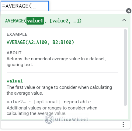
Arguments
| Argument | Requirement | Function |
|---|---|---|
| value1 | Required | The first value or range to consider when calculating the average value |
| value2 | Required | Additional values or ranges to consider when calculating the average value. |
Output
The output AVERAGE(A2:A100, B2:B100) will show the average value for the values in cell range A2:A100 and B2:B100.
8 Easy Methods to Find Average in Google Sheets
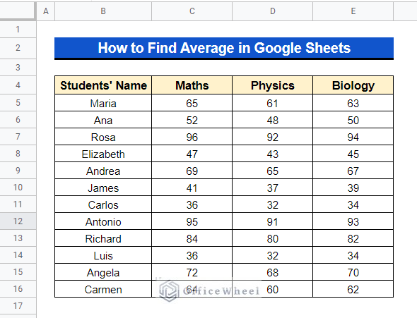
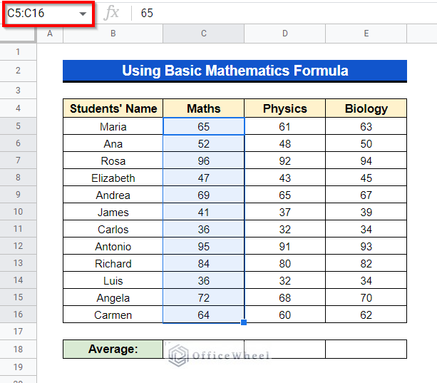
We will use the following sample dataset to demonstrate these methods accurately. The dataset represents some students’ obtained marks in three subjects.
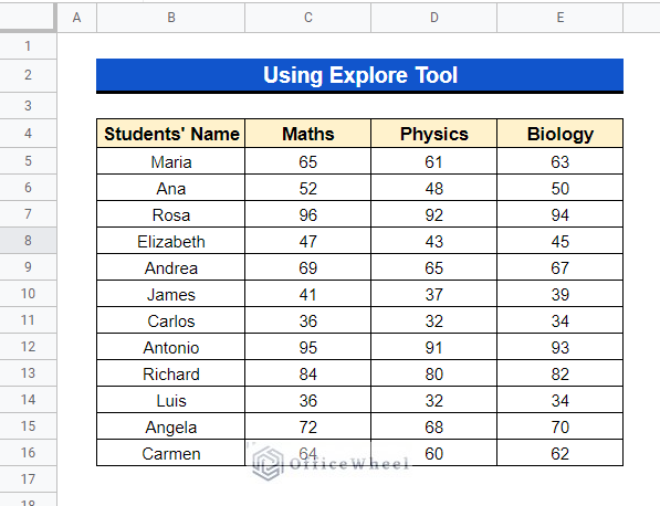
1. Using Explore Tool
The Explore feature in Google Sheets gives us a basic overview of functions that we may use for a particular range of cells. In brief, if we select a range of cells containing numbers, Explore feature will show us the SUM, AVERAGE, MINIMUM, MAXIMUM etc values for the selected range of cells.
Steps:
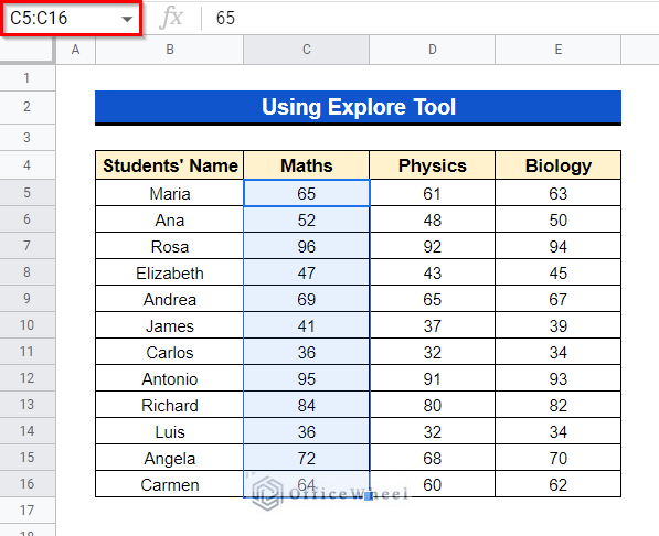
- For example, we will see the AVERAGE of cell range C5:C16 and also C5:E16 in the following dataset.
- First Select cell range C5:C16.
- At the bottom right of the sheet, you will find the option “Explore”.
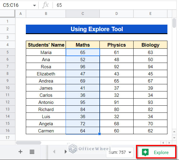
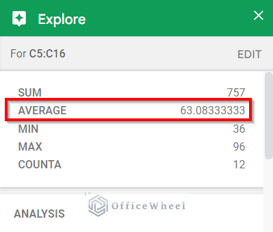
- Press that option and you will see something like this where you will find the AVERAGE value of cell range C5:C16 along with their total SUM, MINIMUM, MAXIMUM values, and the total number of cells that are represented by COUNTA.
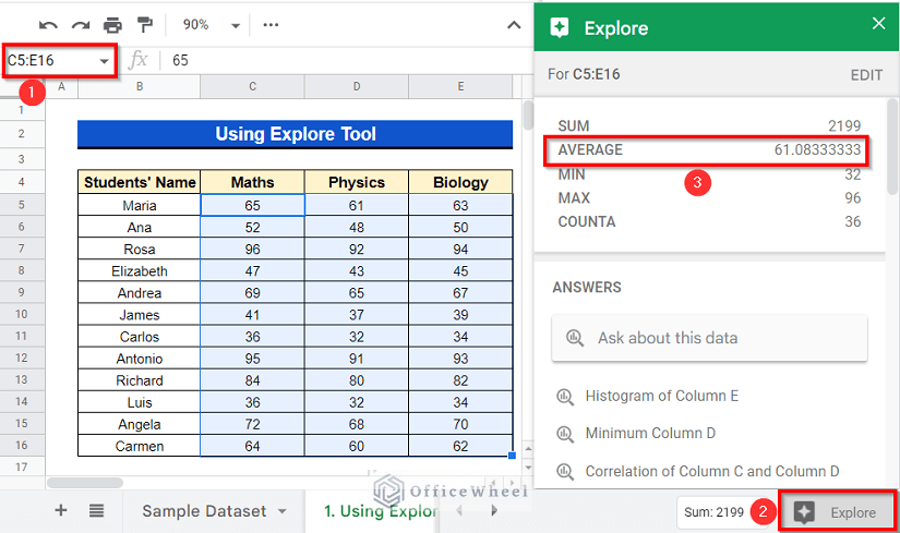
- Now to see the AVERAGE of cell range C5:E16, select the cell range like previously.
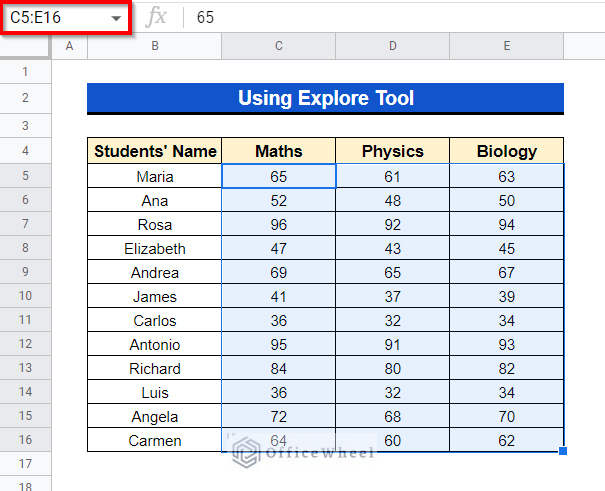
- Then simply use the “Explore” option like previously and you will find the AVERAGE of those cells also.
Read More: How to Average Cells from Different Sheets in Google Sheets
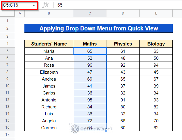
2. Applying Drop Down Menu from Quick View
If we select a particular range of cells containing numbers, a Drop Down menu appears at the bottom right of the sheet where it gives us the Sum, Average, Minimum, Maximum, and total number of cells that is “Count” and the total number of cells containing numbers that is “Count Numbers” for the selected range of cells. If you want to find AVERAGE in Google Sheets within the shortest possible time then this feature is for that.
Steps:
- Select the cell range of numbers whose average you want to know. Here I have selected Cell Range C5:C16.
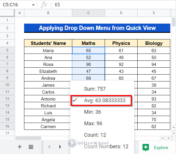
- At the bottom right of the sheet, you will find a Drop Down menu beside the Explore tool.
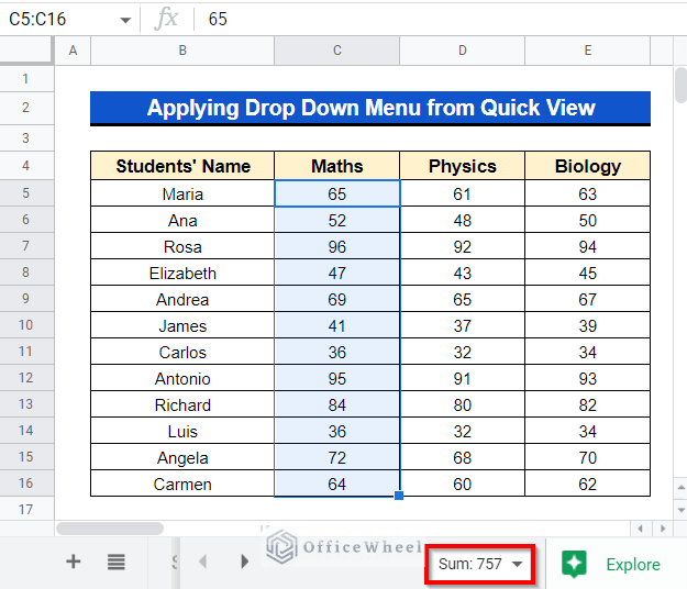
- Click on the Drop Down menu and you will simply get a quick view of the AVERAGE of Cell Range C5:C16. Mark it, and then it will show the average by default whenever you select a range.
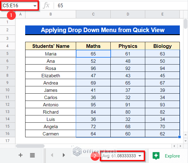
- Like, here I have selected Cell Range C5:E16 and got a quick view of the AVERAGE for those selected cells.
3. Using Basic Mathematics Formula
How do we do the calculation of AVERAGE in our exam? We sum all the values and then divide them by the total number of values. Just like that! We will do the same in Google Sheets also. We can find the AVERAGE in Google sheets using basic mathematics in 2 ways-
3.1 Applying Manual Method
In this method, we will add Cells and divide the sum by the total number of Cells.
Steps:
- Let’s assume, we need to calculate the AVERAGE grade in Maths from the following dataset. The results of students in Maths are shown in Cell Range C5:C16.
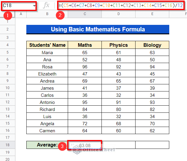
- We selected Cell C18, in which the AVERAGE value will appear. In Cell C18 we will do the following Mathematics and the AVERAGE will be shown in Cell C18.
=(C5+C6+C7+C8+C9+C10+C11+C12+C13+C14+C15+C16)/12
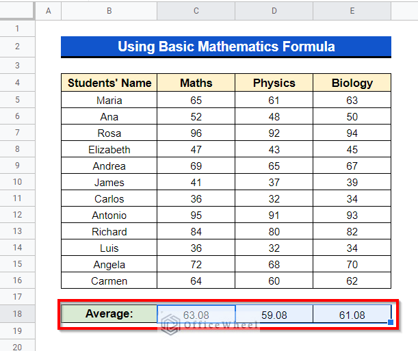
- Now if you want to get the AVERAGES for Physics and Biology, you can do the exact same or you can simply drag right selecting the Fill Handle icon as shown in the circled portion.
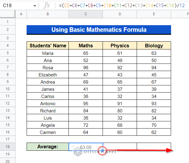
- And you will get the AVERAGE for those also.
3.2 Using SUM Function with Division
If we use the SUM formula then we don’t need to type down Cell numbers or select Cells one by one manually like the previous method.
Steps:
- We can use the SUM function for the same thing. Here like previously, we want to calculate the AVERAGE grade in Maths from the following dataset. The results of students in Maths are shown in Cell range C5:C16.

- We selected Cell C18 like previously, in which the AVERAGE value will appear. In Cell C18 we will apply the following formula-
=SUM(C5:C16)/12
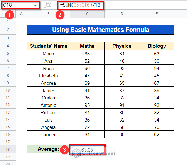
What does the following formula indicate? The SUM function will sum up all the values in Cell Range C5:C16 and then we divide this total sum by 12 because here the number of cells containing numbers is 12.
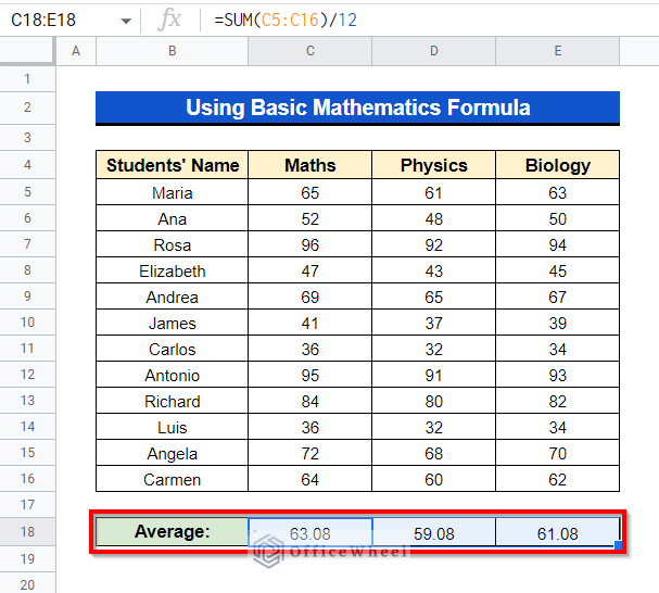
- Then drag right selecting the Fill Handle icon as shown in the circled portion.
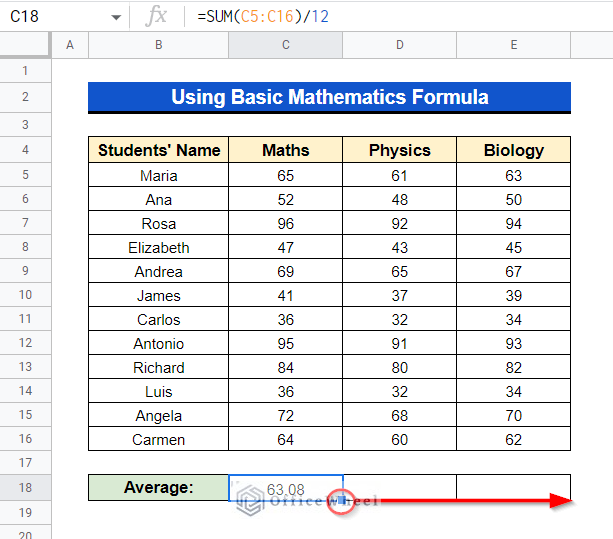
- And you will also receive the AVERAGE for those also.
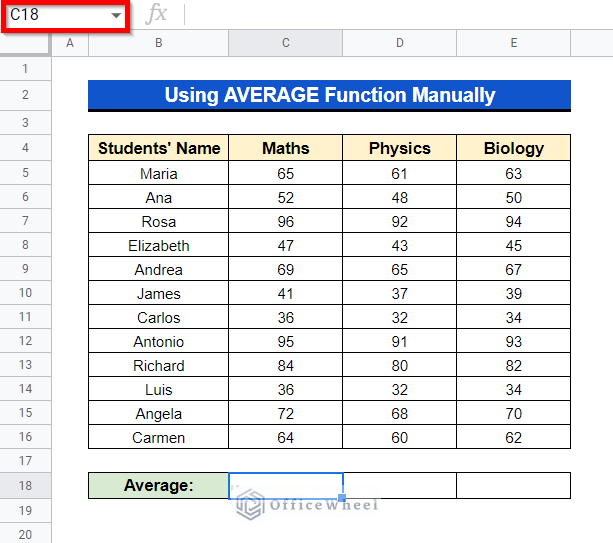
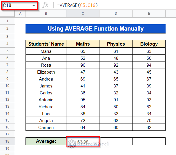
4. Using AVERAGE Function Manually
The built-in AVERAGE function in Google Sheets returns the average of a selected range of cells. And we can use this function manually through a simple process.
Steps:
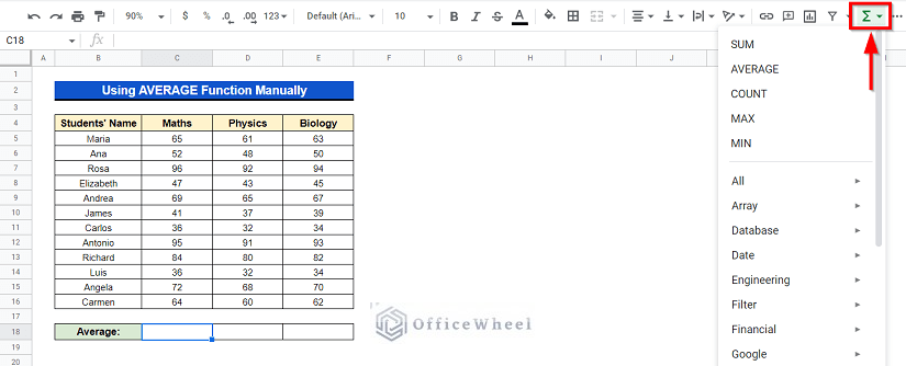
- Suppose, we want to calculate the AVERAGE of Cell Range C5:C16 from the following dataset. First, we selected Cell C18 where the AVERAGE value will appear.
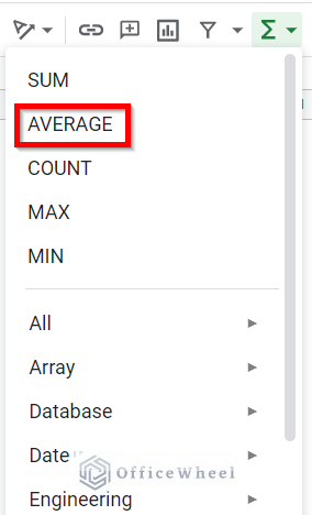
- At the top at Toolbar, press the Sigma “∑” option. This is the Drop Down List of important functions of Google Sheets.
- Select AVERAGE from the Drop Down Menu.
- In Cell C18 the AVERAGE function will appear.
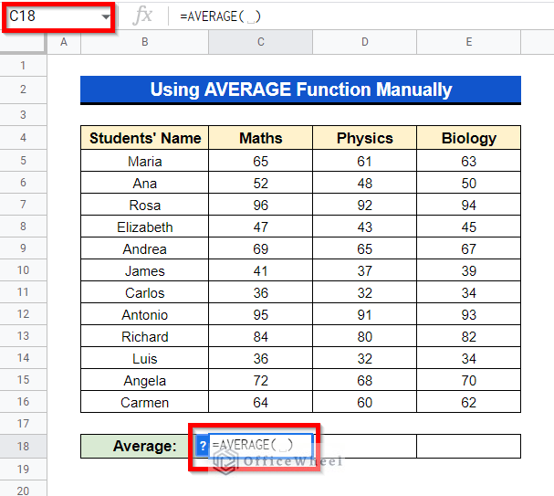
- Now, simply select Cell Range C5:C16.
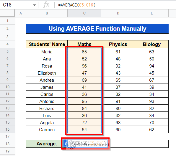
So the final formula will be as follows:
=AVERAGE(C5:C16)
- Finally press Enter. And here is your AVERAGE in Cell C18.
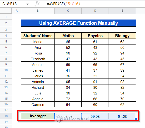
- If you want to get the AVERAGE for the other subjects, you don’t need to do the same again because using the Fill Handle icon just Drag Right.
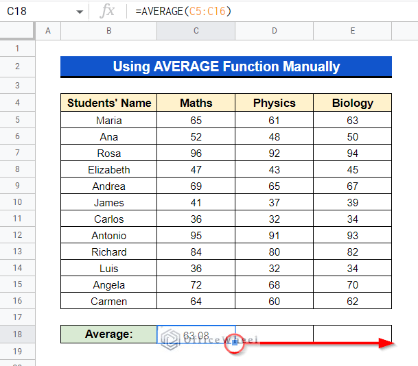
- And here are the AVERAGES of Physics and Biology in Cell D18 and E18 respectively.
5. Applying AVERAGE Function
Using the AVERAGE function will allow us to continue adding values along a column or row or in a range of cells. We don’t have this opportunity for the other methods shown before.
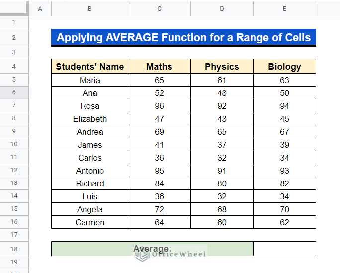
5.1 For a Range of Cells
To perform the AVERAGE function for a range of cells just go through the following steps-
Steps:
- Let’s assume, we want to calculate the AVERAGE mark of the first 5 students in “Maths” from the following dataset.
- In Cell E18 type “=AVERAGE(”.
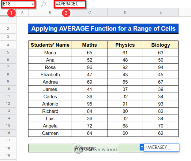
- Select Cell C5, C6, C7, C8 and C9 with pressing Ctrl.
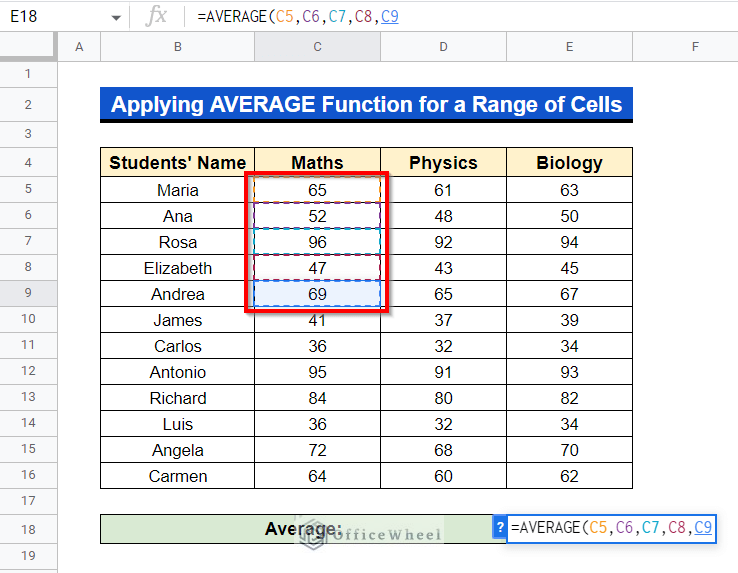
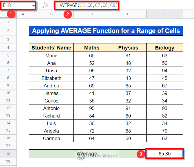
So the final formula will be as follows-
=AVERAGE(C5,C6,C7,C8,C9)
- Now just press Enter and then you will get the AVERAGE in Cell E18.
5.2 For a Column
Basically, the AVERAGE function is used widely to find AVERAGE along a column in Google Sheets.
Steps:
- We will use the following dataset as an example.
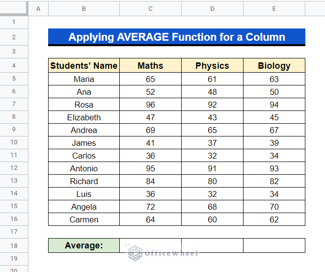
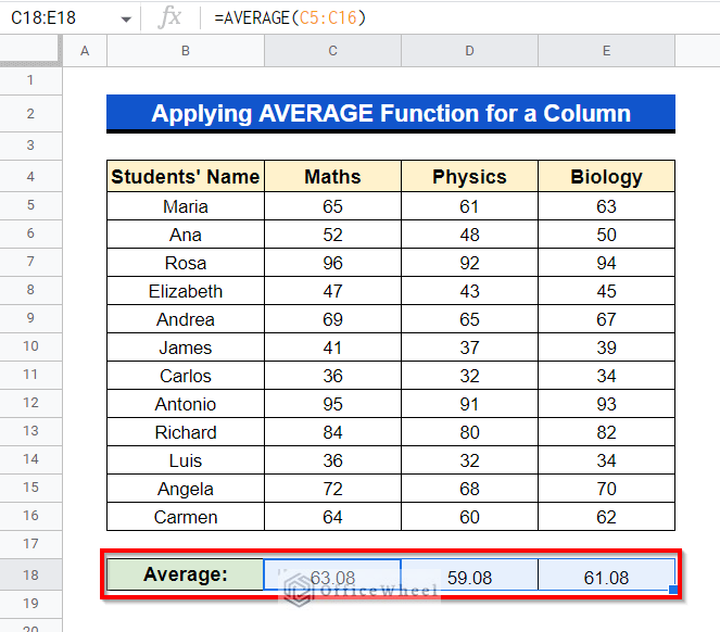
- Here, we will calculate the AVERAGE mark of the students in “Maths”.
- In Cell C18 type “=AVERAGE(” like previously.
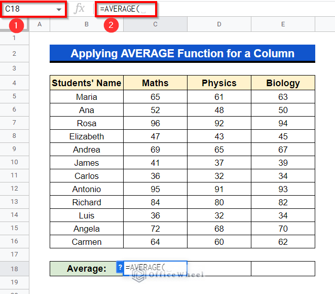
- Select Cell Range C5:C16.
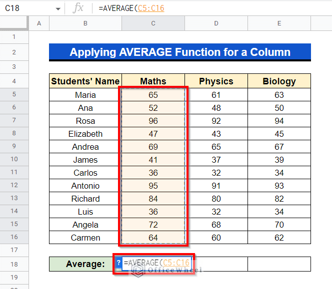
- Press Enter and here is the AVERAGE–
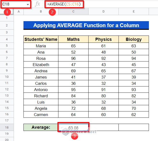
So the final formula will be as follows-
=AVERAGE(C5:C16)
- Now Drag Right using the Fill Handle icon as shown to get the AVERAGE for the other two subjects as well.
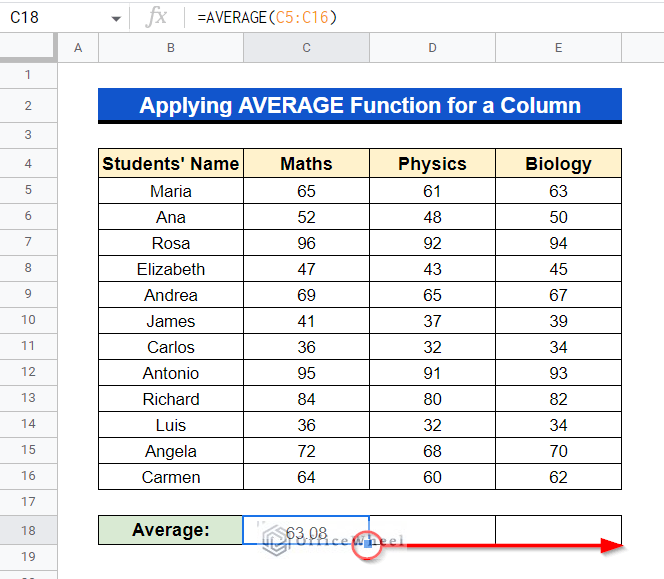
- AVERAGE marks of Physics and Biology will appear in Cell D18 and E18 respectively.
5.3 For a Row
Performing horizontal AVERAGING is as simple as doing it for a column.
Steps:
- In the following dataset, we want to calculate the AVERAGE marks for each of the students.
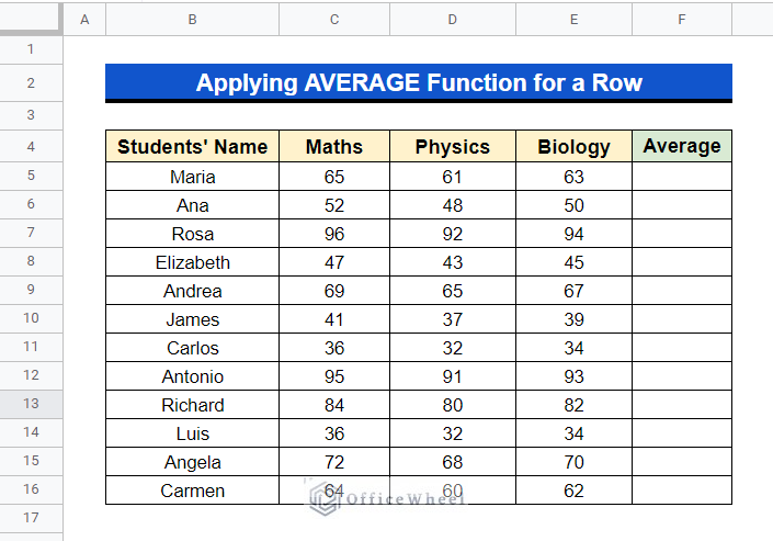
- In Cell F5 simply type “=AVERAGE(” like previously.
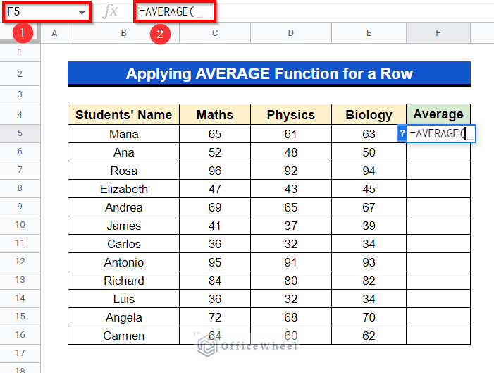
- Select Cell Range C5:E5.
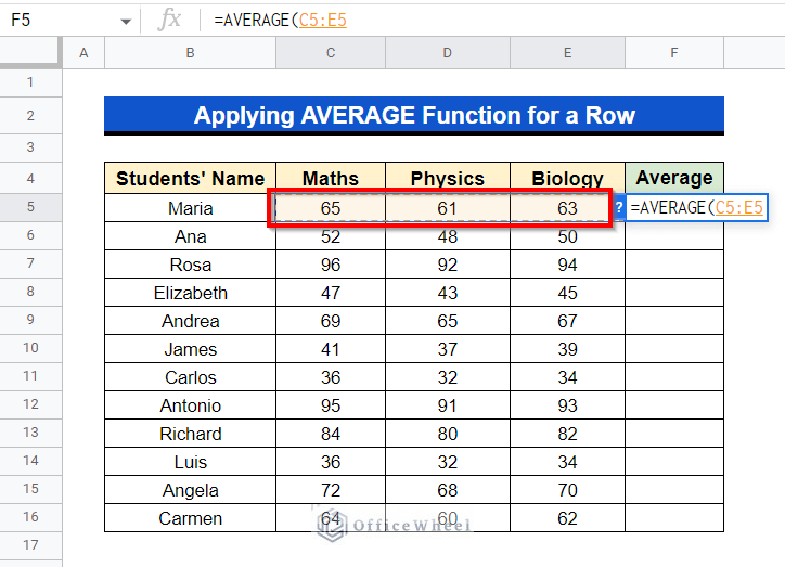
- Press Enter.
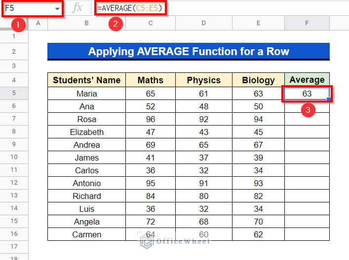
So the final formula will be as follows-
=AVERAGE(C5:E5)
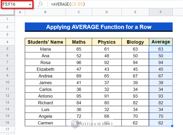
- Drag Down using the Fill Handle icon as shown to get AVERAGE marks of other students as well-
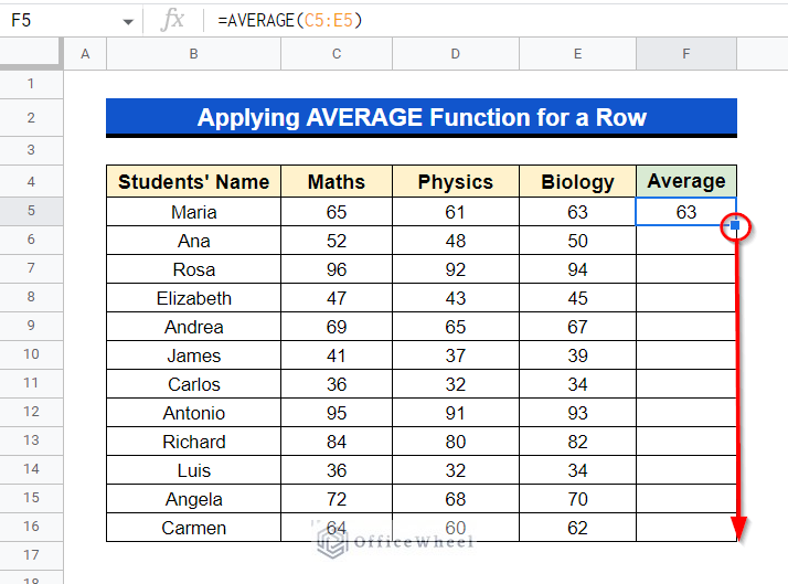
- And all the AVERAGES are calculated along Cell Range F5:F16.
Read More: Calculate Average of Last N Rows in Google Sheets (3 Ways)
5.4 For an Entire Table
Sometimes it is necessary to express the whole progress as an AVERAGE. Finding AVERAGE for an entire table is simple.
Steps:
- Let’s assume, we want to calculate the AVERAGE mark of the students from the following dataset.
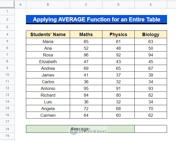
- In Cell E18 type “=AVERAGE(”.
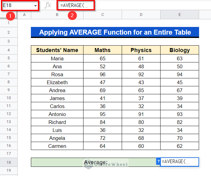
- Select Cell Range C5:E16.
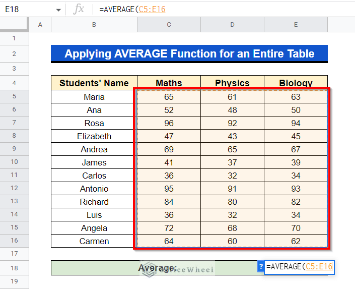
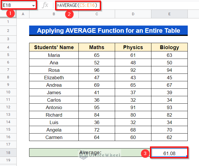
- Simply press Enter and the AVERAGE value will appear in Cell E18.
So the final formula will be as follows-
=AVERAGE(C5:E16)
6. Inserting AVERAGEIF Function
The AVERAGEIF function in Google Sheets returns AVERAGE of a range of cells based on a single criterion.
Steps:
- Assume, from the following dataset, we want to calculate the AVERAGE mark of students in “Maths”.
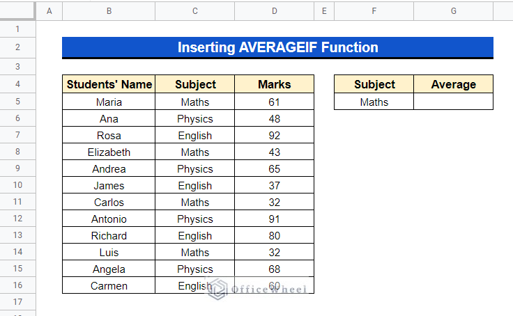
- First, we select Cell G5 where the AVERAGE value will appear. Then we apply the following formula in Cell G5.
=AVERAGEIF(C5:C16,"Maths",D5:D16)
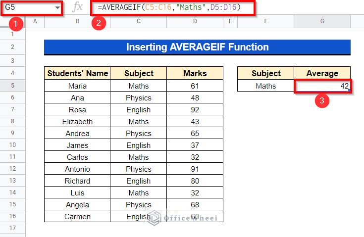
Here, in the formula Cell Range C5:C16 is the Criteria Range from where the function AVERAGEIF will look for the cells for the Criteria subject “Maths”. And cell range D5:D16 is the Average Range from where the function will pick values corresponding to “Maths” and will AVERAGE them.
7. Employing AVERAGEIFS Function
The AVERAGEIFS function in Google Sheets returns AVERAGE of a range of cells based on multiple criteria.
Steps:
- Suppose, from the following dataset, we want to calculate the AVERAGE mark of students in “English” but only for those who obtained more than 40 marks. In Cell G4 we input the word “English” as we want to calculate the AVERAGE of this subject.
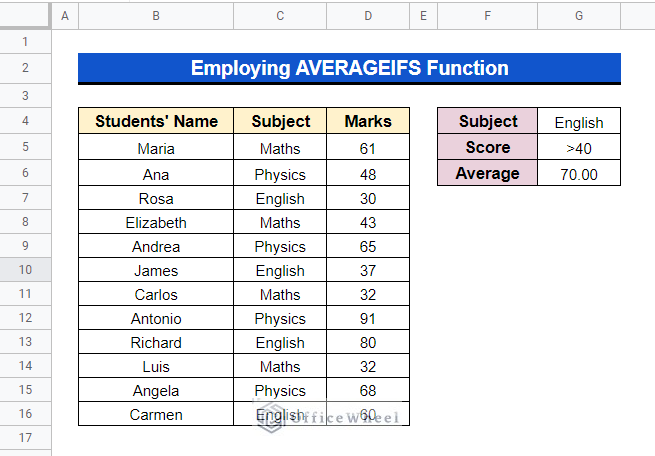
- In Cell G6 apply the following formula and press
=AVERAGEIFS(D5:D16,C5:C16,G4,D5:D16,">40")
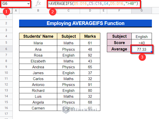
Here, D5:D16 is the Average Range from which the function AVERAGEIFS will pick values based on criterias and AVERAGE them. C5:C16 is the Criteria Range 1 from where the function will look for the Criteria 1 that is “G4”(“English”). D5:D16 is the Criteria range 2 from which the function will look for values corresponding to “English” and also “>40”.
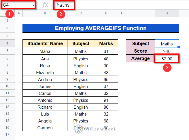
- Now if you want to calculate the AVERAGE mark of students in “Maths” but only for those who obtained more than 40 marks just simply type “Maths” in Cell G4 and see the magic!
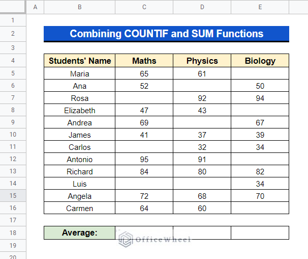
8. Combining COUNTIF and SUM Functions
Previously we have seen some ways of calculating AVERAGE where we used basic mathematics, that is we summed up values from a range of cells and then divided that sum by the number of values. We did the counting of the number of values manually for those methods but if we combine COUNTIF and SUM functions together, we don’t even need to do that!
Steps:
- Presume, we want to calculate the AVERAGE mark of students in “Math” from the following dataset.
- Select Cell C18 where the AVERAGE value will appear. Apply the following formula there and press Enter.
=SUM(C5:C16)/COUNTIF(C5:C16,"<>")
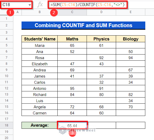
Here, the function SUM sums up the values from Cell Range C5:C16. Then we are using the COUNTIF function for the conditional state. Cell Range C5:C16 is from where the function will pick values following the Criterion “<>” that is if there are any BLANK Cells the COUNTIF function will not count them.
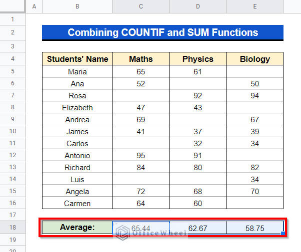
- Now, just Drag Right using the Fill Handle icon as follows to get the AVERAGE for other subjects also.
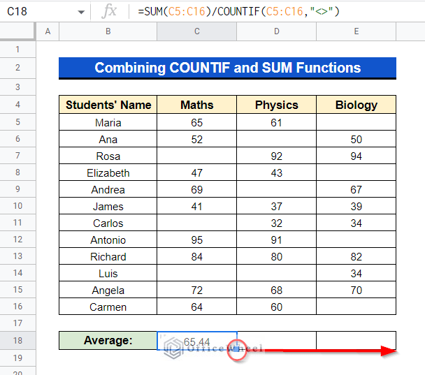
- And that’s it!
Read More: How to Ignore Blank Cells with AVERAGE Formula in Google Sheets
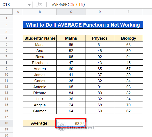
What to Do If AVERAGE Function Is Not Working in Google Sheets?
Sometimes the AVERAGE function may not show the expected result. This can occur for some silly reasons.
1. Format of the Texts
In the following dataset, we are trying to apply the AVERAGE function in Cell C18 for Cell Range C5:C16 but what it is showing is an Error.
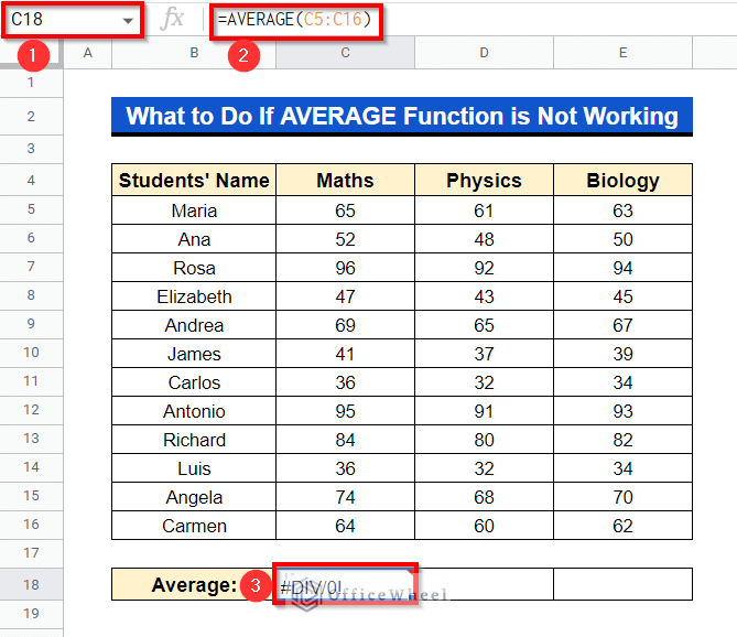
Why is this error occurring? Select the Cell Range C5:C16 and then at the top of your toolbar, select Format.
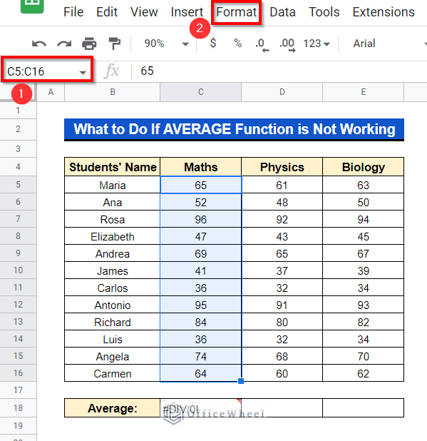
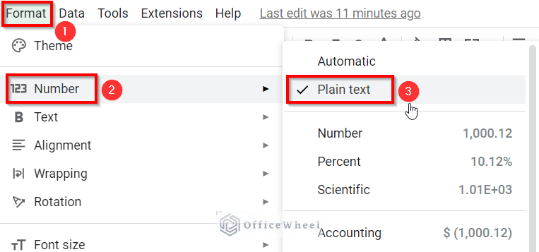
Now see whether the number format is selected as “Automatic” or not. If the number format is selected as “Plain text” then the AVERAGE function won’t work.
Solution:
- Simply select the Cell Range and then go to Format and set the number format as “Automatic”.
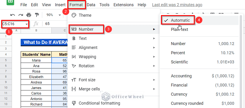
- Now the AVERAGE function will surely gonna work.
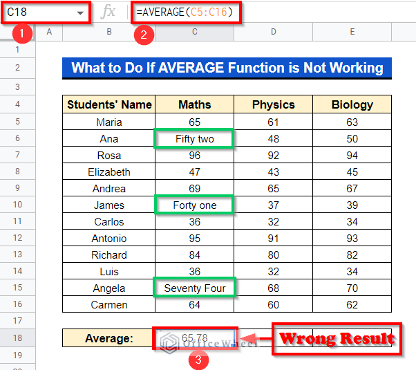
2. Numbers in Words
If a particular Cell Range carries numbers in digits along with numbers in words then the AVERAGE function may work but will show wrong results.
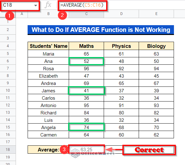
Solution:
- Just try to keep all the numbers in digits and the result will be accurate.
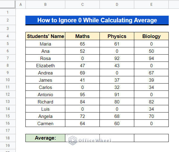
How to Ignore 0 While Calculating Average in Google Sheets?
If we want to ignore Zero “0” while calculating AVERAGE, the AVERAGEIF is simply an outstanding and easy to use function in Google Sheets. So now we’ll show how to find average in Google sheets ignoring zero.
Steps:
- Suppose, we want to calculate the AVERAGE mark of the students in “Maths” excluding those who obtained 0 from the following dataset.
- In Cell C18 apply the following formula and press Enter-
=AVERAGEIF(C5:C16,"<>0")
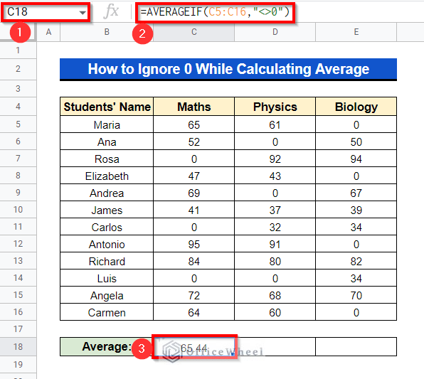
Here, Cell C5:C16 is the Criteria Range from where the AVERAGEIF function will pick the values to calculate AVERAGE, and “<>0” is the Criterion that commands the function not to pick those cells containing “0”.
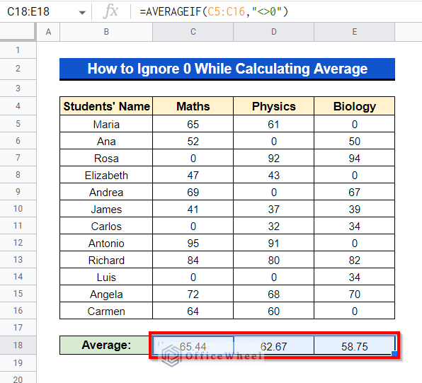
- Now simply Drag Right using the Fill Handle icon as shown in order to perform the same for the other two subjects as well.
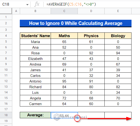
- And the function AVERAGEIF will show the AVERAGES for “Physics” and “Biology” excluding “0” containing cells.
Conclusion
The built in AVERAGE function along with some amazing features like Explore, AVERAGEIF or AVERAGEIFS in Google Sheets will surely gonna help us to do our calculations instantaneously. In this article, we have demonstrated 8 easy methods of how to find AVERAGE in Google Sheets and hope this may help you with your workings. Visit our site officewheel.com for more related articles that might help you.