We frequently need to find the largest value in a column in Google Sheets. The largest value in a data range can be used in numerous instances. Therefore, this article will discuss 7 easy ways to find the largest value in a column in Google Sheets. Also, we’ll demonstrate how to highlight the top 5 values in a column using Conditional Formatting.
A Sample of Practice Spreadsheet
You can copy our practice spreadsheets by clicking on the following link. The spreadsheet contains an overview of the datasheet and an outline of the discussed examples to find the largest value in a column in Google Sheets.
7 Easy Ways to Find Largest Value in Column in Google Sheets
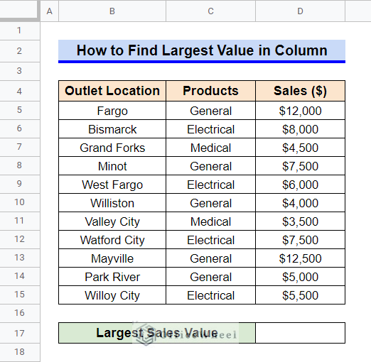
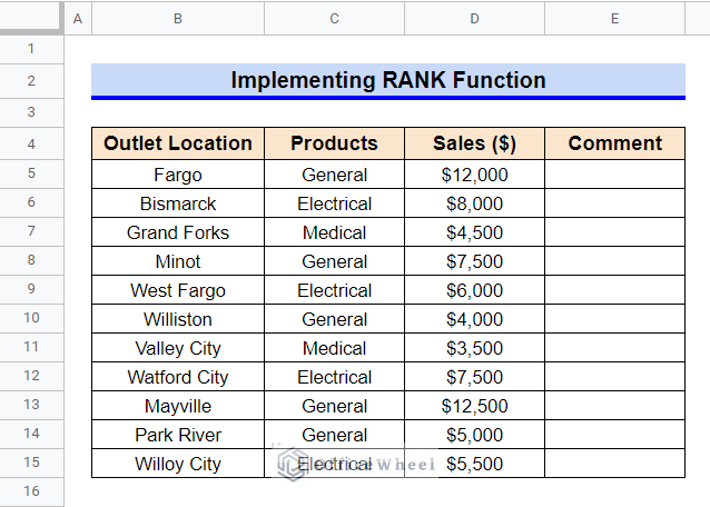
First, let’s get familiar with the dataset that will be used in this article. The dataset contains a list of outlet locations, product types, and sales values for each outlet. We’ll apply a few formulas in Google Sheets to find the largest sales value in the Sales column.
1. Using MAX Function
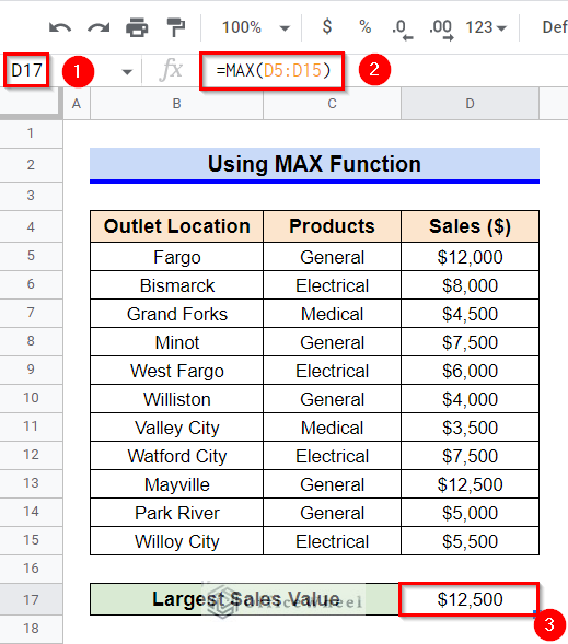
Using the MAX function is perhaps the most customary way to find the largest value in a range. The MAX function can return the maximum value in a numeric dataset.
Steps:
- Firstly, select Cell D17.
- Afterward, type in the following formula-
=MAX(D5:D15)- Finally, get the required output by pressing Enter key.
Read More: How to Find P-Value in Google Sheets (With Quick Steps)
2. Applying LARGE Function
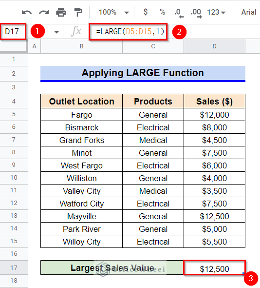
The LARGE function is used for returning the nth largest element from a numeric dataset. Since we require the largest value, we’ll enter the value 1 for the argument n.
Steps:
- First, activate Cell D17 by double-clicking on it.
- Now, insert the following formula-
=LARGE(D5:D15,1)- Later, press the Enter key to get the required output.
3. Employing SORTN Function
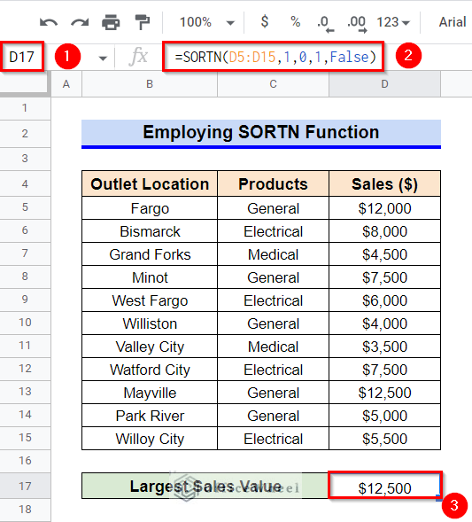
Another function that can help to find the largest value in a column in Google Sheets is the SORTN function. The SORTN function is an exclusive function in Google Sheets and it can return the first n values from a data range after sorting the rows. This function is most useful when we require returning more than one value from a sorted range.
Steps:
- To start, select Cell D17 and then type in the following formula-
=SORTN(D5:D15,1,0,1,False)- Since we require the largest value only, we have inserted the value 1 for argument n. No way is specified for displaying ties by the number 0, the index of the column to be sorted is indicated by the value 1 and the False value sets the sorted range in descending order.
- At this point, get the required output by pressing the Enter key.
Read More: How to Find the Range in Google Sheets (with Quick Steps)
4. Implementing RANK Function
If we require to find the position of the largest value in a column in Google Sheets, then we can apply the RANK function. It is capable of returning the rank of a specified value in a dataset. We have modified our dataset like the following to demonstrate this method.
Steps:
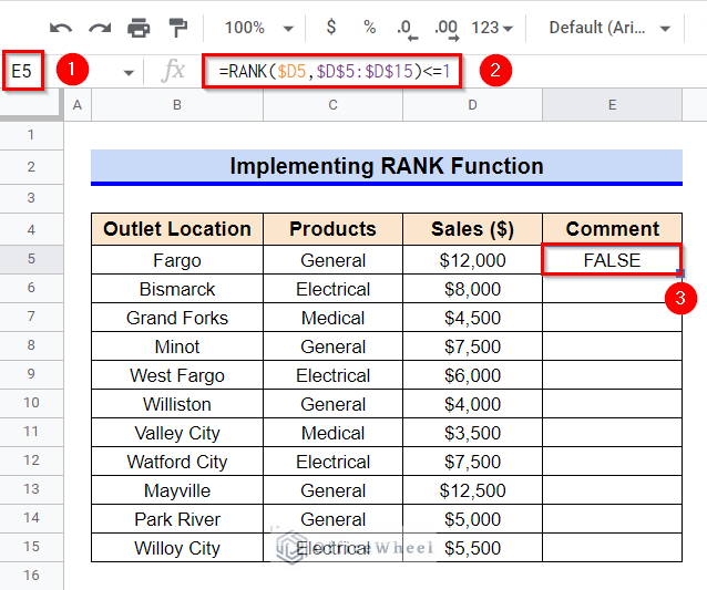
- First, select Cell E5 and activate it by using the function key F2.
- Afterward, insert the following formula-
=RANK($D5,$D$5:$D$15)<=1- If you require the rank of n largest values, just enter the value of n instead of 1 in the formula above.
- Now, press Enter key to get the required output.
- At this time, select Cell E5 again and then hover your mouse pointer above the bottom-right corner of the selected cell. The Fill Handle icon will be visible at this point.
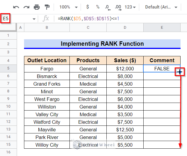
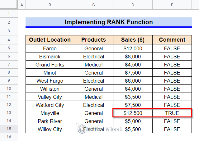
- Use the Fill Handle icon to copy the formula to other cells of Column E. As you can see, the comment is “True” for the subsequent cell with the largest value.
 Read More: How to Use Find and Replace in Column in Google Sheets
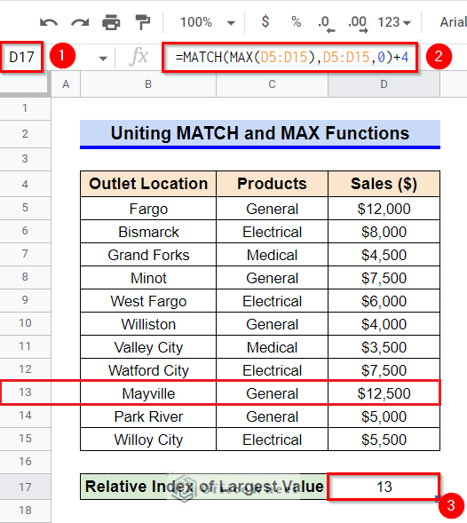
5. Uniting MATCH and MAX Functions
An alternative to using the RANK function to find the position of the largest value in a column is to unite the MATCH and MAX functions. The MATCH function can return the relative position of an item in a specified range if a match is found.
Steps:
- First, activate Cell D17 by double-clicking on it.
- Now, type in the following formula-
=MATCH(MAX(D5:D15),D5:D15,0)+4- Later, press the Enter key to get the required output.
Formula Breakdown
- MAX(D5:D15)
First, the MAX function returns the maximum value in the range D5:D15.
- MATCH(MAX(D5:D15),D5:D15,0)
Later, the MATCH function returns the relative index of the maximum value in the range D5:D15.
- MATCH(MAX(D5:D15),D5:D15,0)+4
Since the MATCH function returns the relative index, we have added 4 (the number of rows prior to the range D5:D15) to get an absolute index.
Read More: Find Value in a Range in Google Sheets (3 Easy Ways)
Similar Readings
- How to Find Edit History in Google Sheets (4 Simple Ways)
- Use FIND Function in Google Sheets (5 Useful Examples)
- How to Find and Delete in Google Sheets (An Easy Guide)
- Find and Replace with Wildcard in Google Sheets
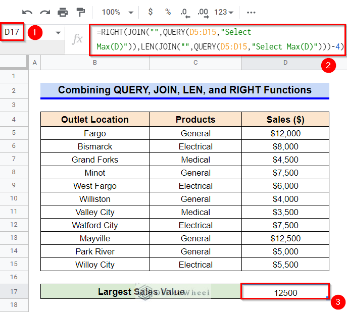
6. Combining QUERY, JOIN, LEN, and RIGHT Functions
Since the QUERY function can perform database-like searching in a dataset and filter data according to a required format, we can use it also to find the largest value in a column in Google Sheets. Here, we’ll also combine the JOIN, LEN, and RIGHT functions with the QUERY function to get the required output.
Steps:
- Firstly, select Cell D17.
- Afterward, type in the following formula-
=RIGHT(JOIN("",QUERY(D5:D15,"Select Max(D)")), LEN(JOIN("",QUERY(D5:D15,"Select Max(D)")))-4)- Finally, get the required output by pressing Enter key.
Formula Breakdown
- QUERY(D5:D15,”Select Max(D)”)
First, the QUERY function runs a Google Visualization API Query Language query across the range D5:D15. The expression Select starts a query. The maximum value in Column D is selected and returned by the specified query. The output of this statement is max and 12500 in two subsequent cells of a column.
- JOIN(“”,QUERY(D5:D15,”Select Max(D)”))
Next, the JOIN function appends all the values returned by the QUERY function. This statement is used twice in the formula and in both instances, it has an output of “max 12500”.
- LEN(JOIN(“”,QUERY(D5:D15,”Select Max(D)”)))-4
Afterward, the LEN function returns the string length of the value joined by the JOIN function. Since we only want to return the largest value, we sub subtracted the value 4 from the length of the appended string length to remove the unwanted part. The output of this part of the formula is 5.
- RIGHT(JOIN(“”,QUERY(D5:D15,”Select Max(D)”)),LEN(JOIN(“”,QUERY(D5:D15,”Select Max(D)”)))-4)
Finally, the RIGHT function returns the 5 rightmost characters from the appended text. The output of this formula is 12500. However, one limitation of this method is that the output is shown as a text value instead of a numeric value.
Read More: Easy Guide to Replace Formula with Value in Google Sheets
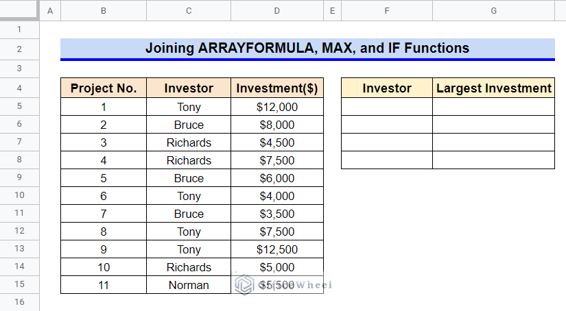
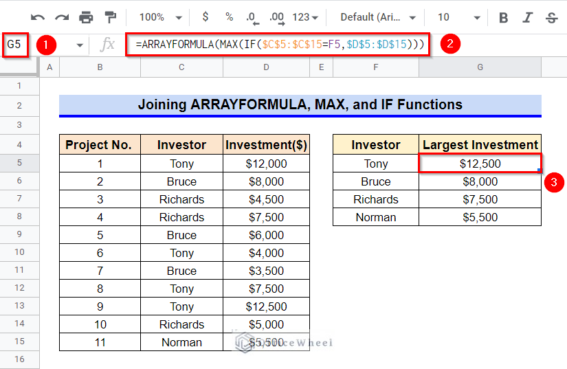
7. Joining ARRAYFORMULA, MAX, and IF Functions
Instead of finding the largest value in a column, sometimes we may require to find the largest value by a group. We require to join the ARRAYFORMULA, MAX, and IF functions for this method. We also require the UNIQUE function to generate a unique list from the dataset below.
Steps:
- First, type in the following formula in Cell F5–
=UNIQUE(C5:C15)- Then, press the Enter key to get a unique range.
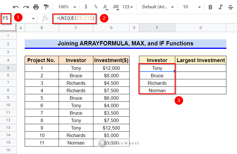
- Afterward, activate Cell G5 and insert the following formula-
=ARRAYFORMULA(MAX(IF($C$5:$C$15=F5,$D$5:$D$15)))- Now, get the required output by first pressing the Enter key and then using the Fill Handle icon.
Formula Breakdown
- IF($C$5:$C$15=F5,$D$5:$D$15)
To start, the IF function first checks whether any value in the range C5:C15 is equal to the content of Cell F5. If any match is found, then the IF function returns the subsequent value from the range D5:D15.
- MAX(IF($C$5:$C$15=F5,$D$5:$D$15)
Later, the MAX function returns the maximum value from the set of values returned by the IF function.
- ARRAYFORMULA(MAX(IF($C$5:$C$15=F5,$D$5:$D$15)))
Here, the ARRAYFORMULA function helps the non-array function IF to deal with an array.
Read More: Find All Cells With Value in Google Sheets (An Easy Guide)
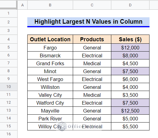
How to Highlight Largest N Values in Google Sheets
We can use the Conditional Formatting tool to highlight a required number of values from a data range. This will help us to easily find our required data in a dataset. Here, we’ll use the Conditional Formatting tool to highlight and find the largest 5 values in a column in Google Sheets.
Steps:
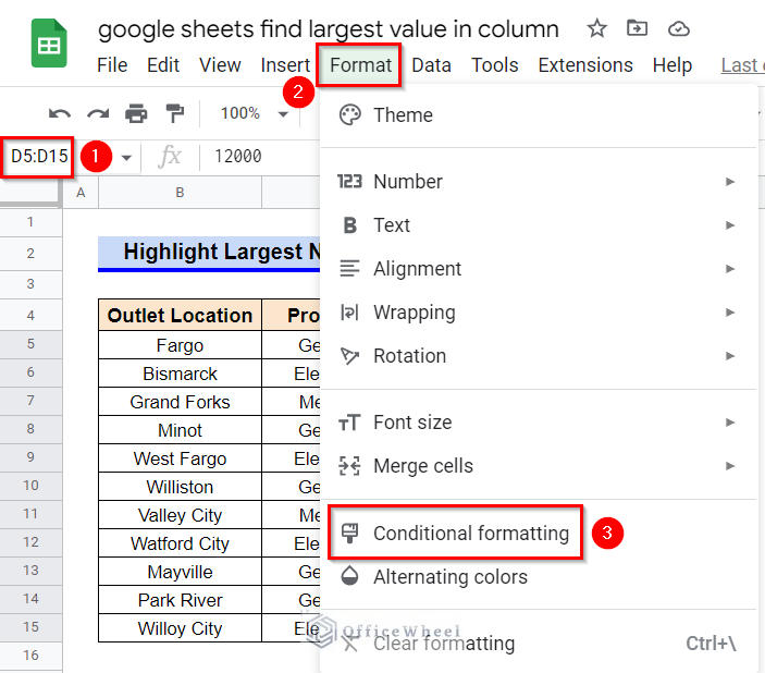
- First, select the range D5:D15 and then go to the Format ribbon.
- Select the Conditional Formatting tool from the appeared options.
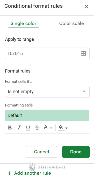
- A sidebar like the following will appear.
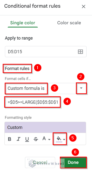
- Now, set the Format Rules to Custom Formula from the dropdown list.
- Afterward, set the formula to the following-
=$D5>=LARGE($D$5:$D$15,5)- Consequently, select the required fill color from Formatting Style.
- And now, click on Done.
- The cells that contain the largest 5 values in the column have now been highlighted.
Conclusion
This concludes our article to learn how to find the largest value in a column in Google Sheets. I hope the demonstrated examples were ideal for your requirements. Feel free to leave your thoughts on the article in the comment box. Visit our website OfficeWheel.com for more helpful articles.
Related Articles
- How to Find Median in Google Sheets (2 Easy Ways)
- Find Hidden Rows in Google Sheets (2 Simple Ways)
- How to Find Slope of Graph in Google Sheets (With Easy Steps)
- Find Uncertainty of Slope in Google Sheets (3 Quick Steps)
- How to Find Linear Regression in Google Sheets (3 Methods)
- Find Frequency in Google Sheets (2 Easy Methods)
- How to Find Slope of Trendline in Google Sheets (4 Simple Ways)