While working on google sheets sometimes you need to extract some particular characters, Capital letters, decimal numbers, and so on. But Getting all this method done manually is very time-consuming and quite difficult. Here, we will learn how to use the REGEXEXTRACT function between two characters in google sheets using simple and practical examples. So, let’s start.
A Sample of Practice Spreadsheet
You may copy the spreadsheet below and practice by yourself.
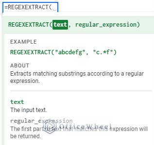
Introduction to the REGEXEXTRACT Function in Google Sheets
The REGEXEXTRACT function returns the texts in a string. The REGEXEXTRACT function extracts individual texts from a string and shows the texts as output. For example, suppose the actual Text is “Here is a beautiful Bird” then the output will be H as the REGEXEXTRACT function extracts individual characters from a string.
Syntax
REGEXETRACT (text, regular_expression )
Inputs
| ARGUMENT | REQUIREMENT | Sample heading |
|---|---|---|
| text | Required | The input of the total text. |
| regular_expression | Optional/ Required | The characters of the expression will be returned. |
Return Value
Returns the exact match from the actual text.
12 Practical Examples of Using REGEXEXTRACT Function Between Two Characters in Google Sheets
Here, follow the simple examples to learn about using the Google Sheets REGEXEXTRACT function between two characters.
1. Extracting Between Two Characters
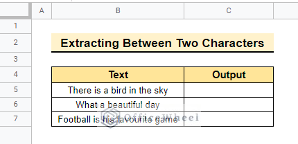
Here, we will use the REGEXEXTRACT function to extract the actual character in the dataset between two random characters using the below dataset.
Follow the steps below to execute this method.
📌 Steps:
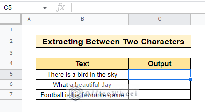
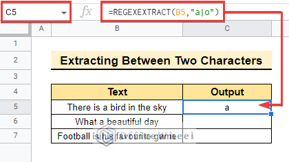
- First, Select cell C5 to enter the REGEXEXTRACT function.
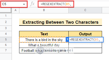
- Then, enter the function and select cell B5 for the actual test or manually write down the text and close it with double quotes.
- After that, write down two characters manually using (|) to select either of the characters which is in the text and close this part with double quotes as below.
- So, the overall formula is,
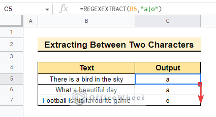
=REGEXEXTRACT(B5,"a|o")- As the text contains “a” the output is “a”.
- Now, drag down the fill handle and copy the formula into every blank cell of the dataset.
2. Pulling Out Single Characters
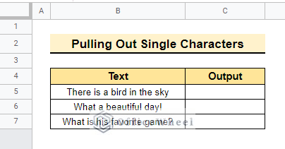
Now, we will use the REGEXEXTRACT function between two characters for pulling out single characters using the dataset below.
📌 Steps:
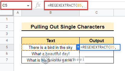
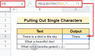
- Initially, select cell C5 to enter the formula.
- And, select cell B5 to get the text, or write down the total text manually and enclose it with double quotes as before.
- Therefore, insert 5 dots to represent 5 characters in a word and close it with double quotes.
- Find the formula below,
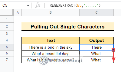
=REGEXEXTRACT(B5,".....")- Finally, drag down the fill handle and copy the same formula in the other cell.
3. Bringing out Numbers
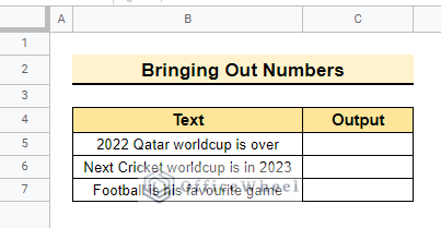
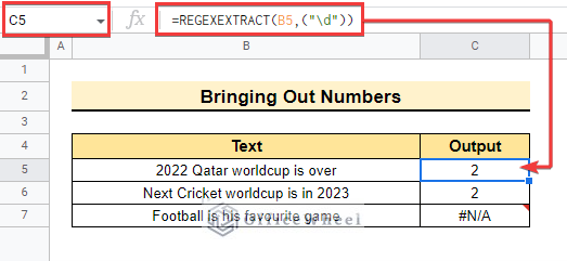
We will use the REGEXEXTRACT function between two characters to bring out numbers from the text using the below dataset. Let’s start.
📌 Steps:
- In the beginning, select cell C5 to enter the formula as before
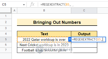
- Moreover, enter the formula and select cell B5 to get the text as below.
- After that, write down “d” manually to get the decimal number along with \ to get the number as below.
- Now, the formula,
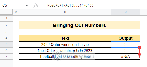
=REGEXEXTRACT(B5,("\d"))- Now, drag down the fill handle as before to copy the formula in every cell.
- It is visible that the output will be shown as #N/A if there is no number in the text.
If we add a plus after d then it will show the total number from the dataset.
Read More: How to Find Unique Values Between 2 Columns in Google Sheets
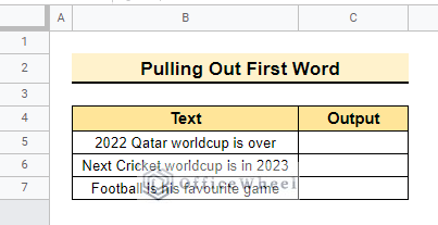
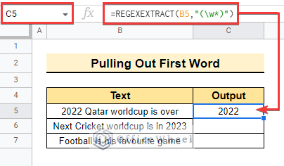
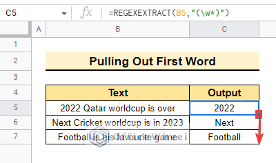
4. Pulling out First Word
Step-by-step procedure of using the REGEXEXTRACT function between two characters to pull out the first word with the below dataset.
📌 Steps:
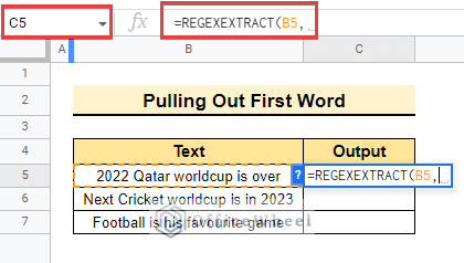
- Now, select cell C5 to enter the function and then select cell B5 to get the whole test as a lookup value.
- Now write down (\w*) to get the first word as below.
- Here, the formula is as follows
=REGEXEXTRACT(B5,"(\w*)")- Lastly, drag down the fill handle to copy the formula in the other cell.
Read More: How to Remove Spaces Between Words in Google Sheets
Similar Readings
- How to Find Correlation Between Two Columns in Google Sheets
- Insert Rows Between Other Rows in Google Sheets (4 Easy Ways)
- How to Calculate Time Between Dates in Google Sheets (6 Ways)
- Find Difference Between Two Columns in Calculated Field of Google Sheets Pivot Table
- How to Filter Between Two Dates in Google Sheets
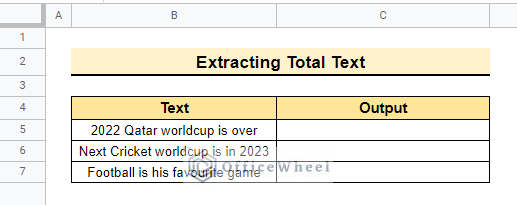
5. Extracting Total Text
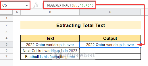
Here, We will extract the total text using the REGEXEXTRACT function between two characters with the below dataset.
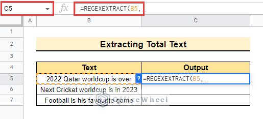
📌 Steps:
- First, complete the steps already described to get the text.
- Now, write (.) and add a (+) sign with it so that the total text will be copied.
- So, the overall formula is below,
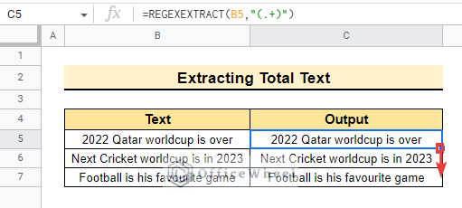
=REGEXEXTRACT(B5,"(.+)")- Furthermore, drag down the fill handle to copy the formula.
Read More: Generate Random Numbers or Text Between Limits in Google Sheets
6. Taking out the Middle Character
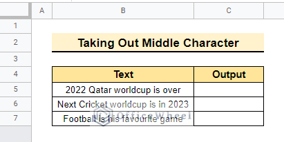
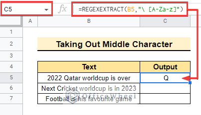
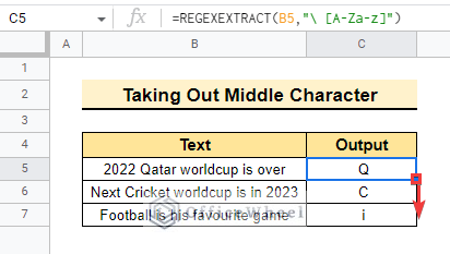
Follow the step-by-step procedure to use the REGEXEXTRACT function between two characters in case of taking out the middle character using the dataset below.
📌 Steps:
- In the beginning, select the text as the way is already shown before.
- Correspondingly, write down [A-Za-z] and put a blank space before. So, it covers everything except the first word.
- As a result, the formula is,
=REGEXEXTRACT(B5,"\ [A-Za-z]")- Lastly, drag the fill handle and execute the method.
7. Finding and Matching Particular Word
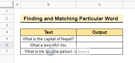
The dataset below contains text and now we will extract a particular word using the REGEXEXTRACT function between two characters with the dataset below.
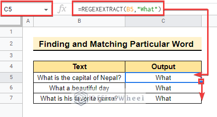
- Here, enter the formula into cell C5 and select B5 as the lookup value.
- Now, to match the value with the text write the particular word and enclose the word with a double quote.
- Finally, drag down the fill handle and complete the method as below.
- Here, the output of the formula is as below
=REGEXEXTRACT(B5,"What")8. Extracting both the Numbers and Preceding Characters
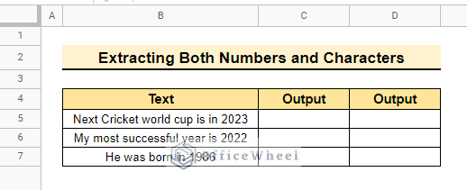
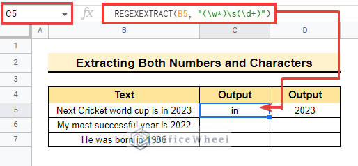
Here, we will extract both the number and preceding characters at the same time. The below dataset contains text with numbers and characters.
📌 Steps:
- Clearly, at first, enter the formula into cell C5 and select cell B5 as the lookup value.
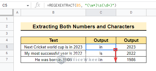
- Therefore, write “(\w*)\s(\d+)” so that it returns both the number and character as below but this formula will return only the previous character of the number.
- Overall formula,
=REGEXEXTRACT(B5, "(\w*)\s(\d+)")- Finally, drag down the fill handle and copy the formula.
Read More: Google Sheets Count Cells Between Two Numbers with COUNTIF Function
Similar Readings
- How to Move Between Tabs in Google Sheets (3 Easy Ways)
- Calculate Number of Years Between Two Dates in Google Sheets
- How to Use IF Condition Between Two Numbers in Google Sheets
- Difference Between COUNT and COUNTA in Google Sheets
- How to Link Cells Between Tabs in Google Sheets (2 Examples)
9. Finding Capital Letter
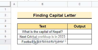
Now, we will execute the method of finding capital letters in the text using the REGEXEXTRACT function between two characters. The dataset is below.
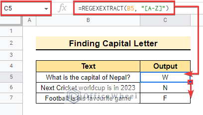
- After that select cell B5 as a lookup value into cell.
- Moreover, write [A-Z] so that the formula returns to the first capital letter in the dataset, and then drag down the fill handle to complete the formula.
- Now the formula is below
=REGEXEXTRACT(B5, "[A-Z]")10. Pulling out Small Letter
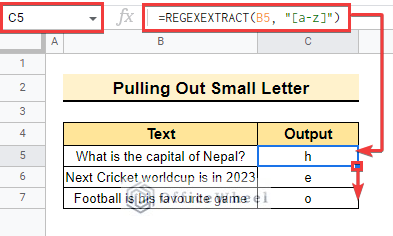
Here, we will pull out small letters using the REGEXEXTRACT function with the same dataset.
Now follow the steps below to execute this method.
📌 Steps:
- In the beginning, execute the formula as shown in the previous method.
- But, we will use [a-z] instead of [A-Z] to get the return of the first small letter in the text.
- So, the overall formula will be the following
=REGEXEXTRACT(B5, "[a-z]")- As a result, we will get the first small letter from the selected text.
- Following, drag the fill handle below to get a similar result for all texts.
11. Extracting Characters from Group
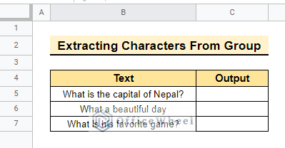
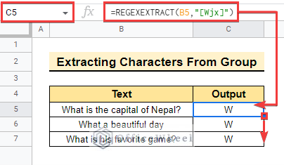
We will extract the existing character of the text from a group of random characters using the REGEXEXTRACT function. The dataset is below. Now, we want to extract characters from our determined group “Wjx” here. Follow the steps below to do this.
📌 Steps:
- Initially, enter the formula into cell C5 and use the lookup text as cell
- Consequently, write down a random group of letters and enclose it with double quotes.
- Complete the formula and drag down the fill handle to complete the method.
- Here, the overall formula,
=REGEXEXTRACT(B5,"[Wjx]")12. Taking out Decimal Numbers
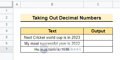
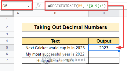
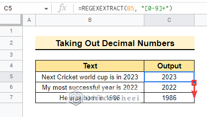
Here, we will use the REGEXEXTRACT function to take out the decimal numbers from the text using the dataset below.
📌 Steps:
- In the beginning, select cell C5 and enter the formula.
- Then, select cell B5 as the lookup text and write down [0-9] so that it returns to the decimal numbers only.
- So, the formula is below,
=REGEXEXTRACT(B5, "[0-9]+")- In the end, drag down the fill handle and complete the method.
Finding a number is already shown before but this method is easier than the other one and easy to extract.
Things to Remember
- Always enclose text with double quotes while implementing the method.
- Both numbers and letters can be extracted together using the REGEXEXTRACT function.
Conclusion
In this article, we explained how to use the REGEXEXTRACT function between two characters in Google Sheets in different ways. Hopefully, the methods will help you to apply the function to your own dataset. Please let us know in the comment section if you have any further queries or suggestions. You may also visit our OfficeWheel blog to explore more Google Sheets-related articles.
Related Articles
- How to Calculate Hours Between Two Times in Google Sheets
- Find Number of Months Between Two Dates in Google Sheets
- How to Find Missing Values Between Two Columns in Google Sheets
- Conditional Formatting Between Two Values in Google Sheets
- How to Insert Lines Between Cells in Google Sheets
- Calculate Percentage Difference Between Two Numbers in Google Sheets
- How to SUMIF Between Two Dates in Google Sheets (3 Ways)

