Find Difference Between Two Columns in Calculated Field of Google Sheets Pivot Table

The Pivot Table is a dynamic feature in Google Sheets. We can do several calculations by using it. Sometimes we need to obtain the difference between two columns in the Calculated Field of the Pivot Table. So in this article, we’ll see 2 suitable ways to find the difference between two columns in the Calculated Field of Google Sheets Pivot Table with clear steps and images.

A Sample of Practice Spreadsheet

You can download Google Sheets from here and practice very quickly.

2 Suitable Ways to Find Difference Between Two Columns in Calculated Field of Google Sheets Pivot Table

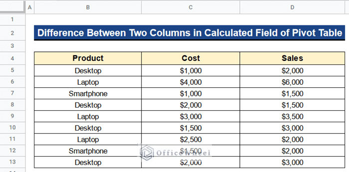
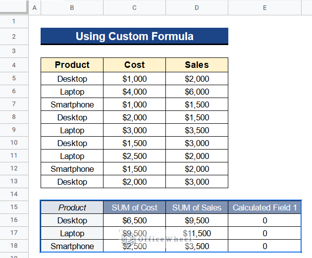
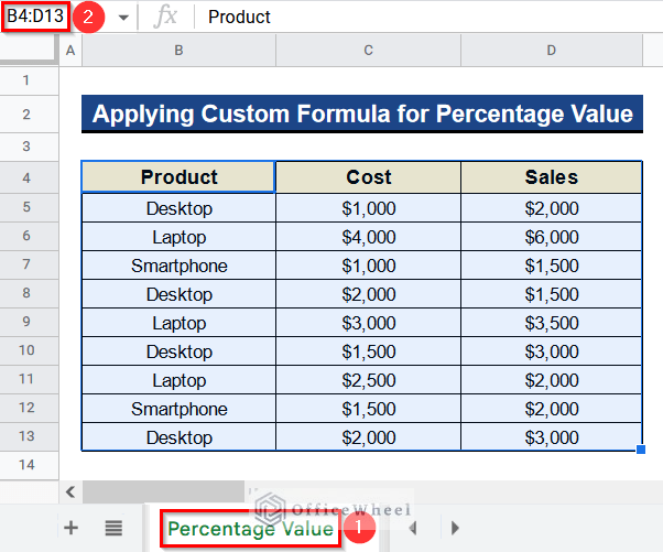
Let’s get introduced to our dataset first. Here we have some products in Column B, their cost prices in Column C, and their sales prices in Column D. Now we want the difference between the sales price and cost price which is the profit of the products. So, I’ll show you 2 suitable ways to find the difference between two columns in the Calculated Field of Google Sheets Pivot Table using this dataset.

1. Using Custom Formula

In the beginning, we’ll use a custom formula in our method. By using this formula we’ll get the difference between two columns, Columns C and D in the Calculated Field of Google Sheets Pivot Table. The formula is very simple. We’ll just subtract the cost prices from the sales prices of the products and then get the profits quickly. Let’s see the steps.

Steps:

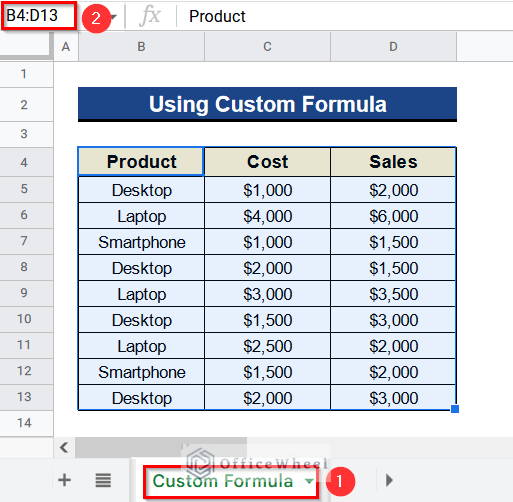
• Firstly, rename the current sheet as Custom Formula and select the cells from Cell B4 to D13.

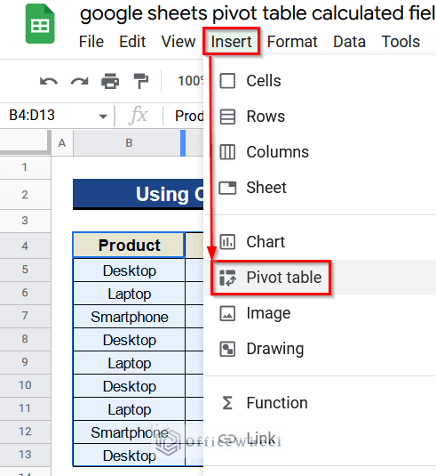
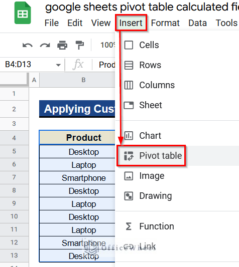
• Now, we have to create a Pivot Table so go to Insert > Pivot Table.

• Then, Create Pivot Table window will open.
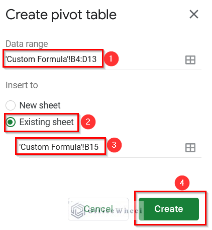
• Secondly, the Pivot Table will automatically show the range from Cell B4 to D13 in the Data Range menu.
• Next, select the radio button beside the Existing Sheet option and give the position of the Pivot Table in Cell B15.
• After that, press the Create button.

• The Pivot Table Editor window will open now.
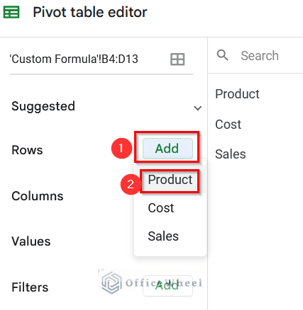
• Thereafter, select the Add button in the Rows menu and add Product from there.

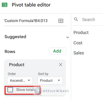
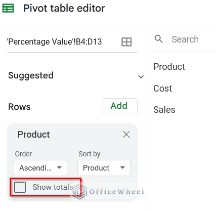
• Afterward, untick the box beside Show Totals in the Rows menu.

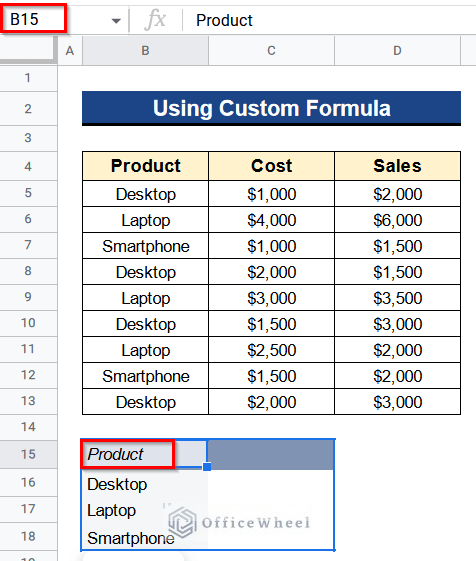
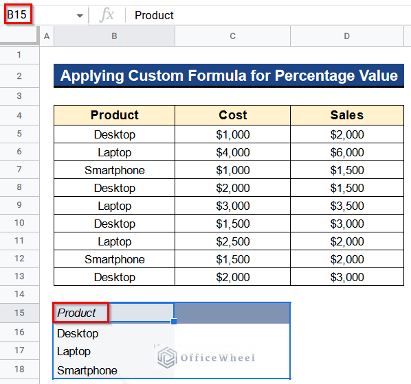
• Consequently, you’ll get a Pivot Table starting from Cell B15 with the unique products list.

• Again, go to the Pivot Table Editor window.
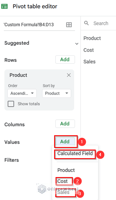
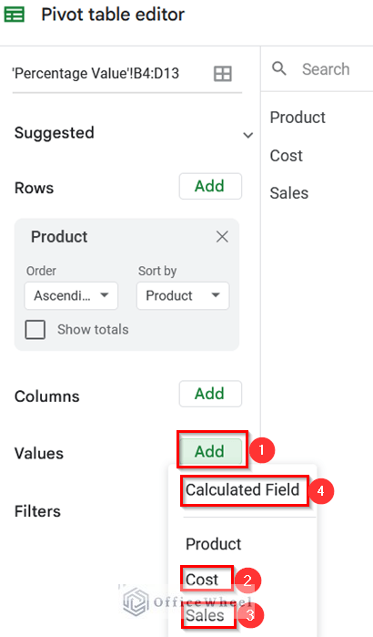
• Moreover, add Cost, Sales, and Calculated Field serially in the Values menu.

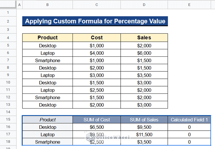
• Further, you’ll get the total cost prices of the products in Column C, the total sales prices of the products in Column D, and Calculated Field 1 in Column E.
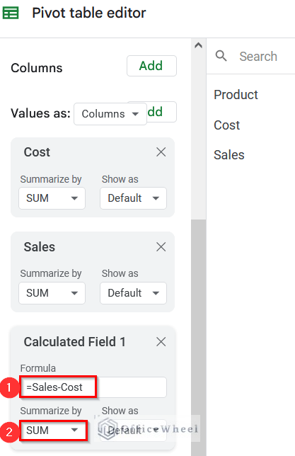
• Now, we’ll insert our formula in the Calculated Field 1 to get the profit of the products.

• At this time go to the Pivot Table Editor window.
• Apart from this, write the following formula in the formula box under the Calculated Field 1 menu-

• Also, select SUM under the Summarize By menu.

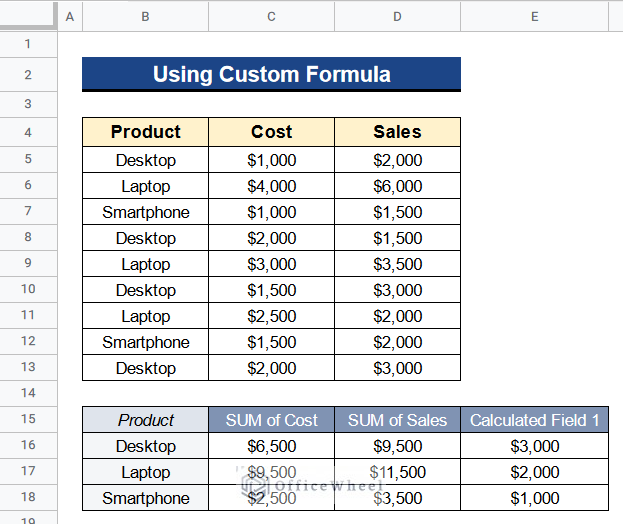
• Then, you’ll find the profit easily in Column E.

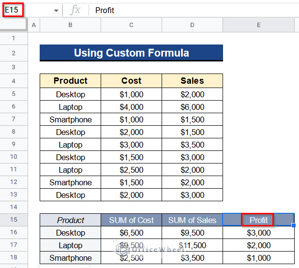
• Finally, rename Cell E15 as Profit from Calculated Field 1.
• At last, you’ll get your desired values in Column E where we are showing the difference between two columns, Columns C and D as profit in the Calculated Field of Google Sheets Pivot Table.

Read More: How to Find Unique Values Between 2 Columns in Google Sheets

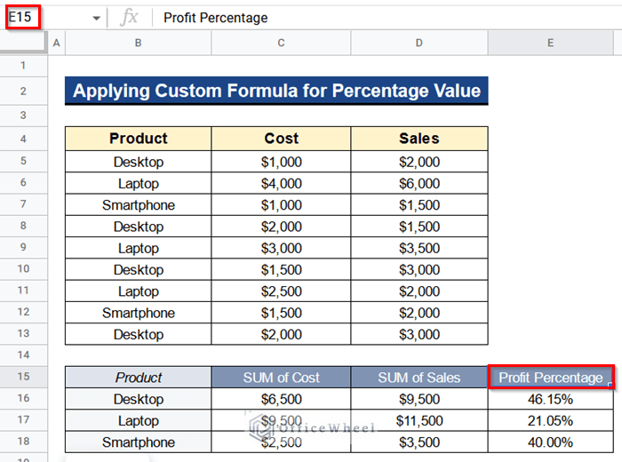
2. Applying Custom Formula for Percentage Value

We’ll look into a different problem now. We want the difference between the two columns carrying cost prices and sales prices of the products as a percentage value. Because in the real scenario the percentage value of profit is more widely used than the simple profit. For this reason, I’ll change the custom formula a little bit. We’ll divide the profit by the cost price to get the percentage profit of the products. Let’s see how to do it.

Steps:

• First of all, rename the sheet as Percentage Value and select the cells from Cell B4 to D13 which is our dataset.

• Then, go to Insert > Pivot Table to create the table.

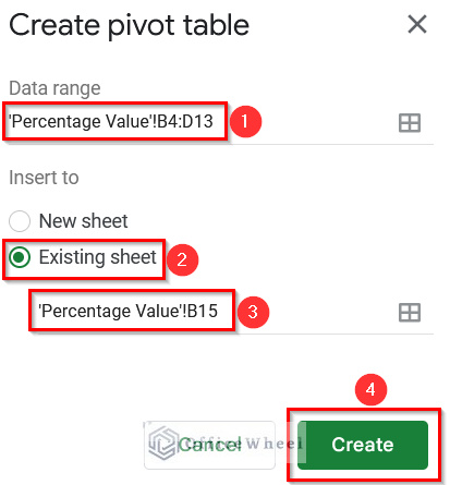
• Next, you’ll see the range from Cell B4 to D13 is automatically there in the Data Range menu under the Create Pivot Table window.
• After that, select the Existing Sheet option and put Cell B15 as the position of the Pivot Table.
• Also, click on the Create button to create the Pivot Table.

• Again the Pivot Table Editor window will open.
• Afterward, add Product in the Rows menu.

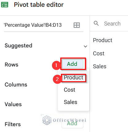
• Consequently, don’t forget to untick the Show Totals option in the Rows menu.

• Further, there will be a Pivot Table starting from Cell B15 having the unique products list.

• Apart from this, add Cost, Sales, and Calculated Field one by one in the Values menu from the Pivot Table Editor window.

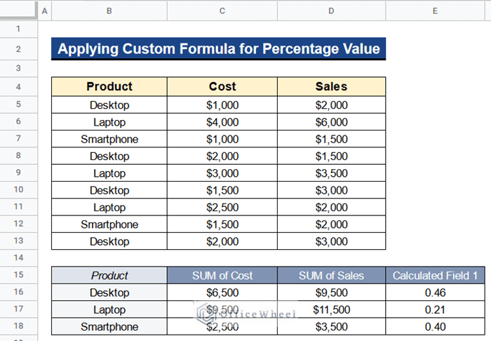
• Then, the total cost prices of the products, total sales prices of the products, and the Calculated Field 1 will be in Columns C, D, and E respectively.
• Next, I’ll put a formula in the Calculated Field 1 to get the profit percentage of the products.

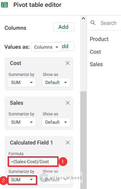
• To insert the formula go to the Pivot Table Editor window and type the following formula in the formula box under the Calculated Field 1 menu-

• Moreover, don’t forget to select SUM under the Summarize By menu.

• You’ll get the results in Column E in the decimal number format. But we want the profit percentage in the percentage format.

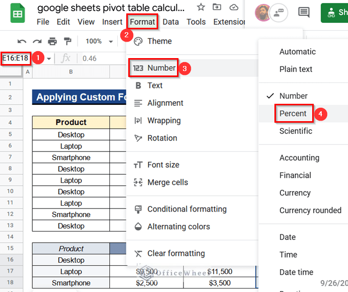
• For that purpose, select Cells E16 to E18 and go to Format > Number > Percent.

• Ultimately, the output is now in the percentage format in Column E.

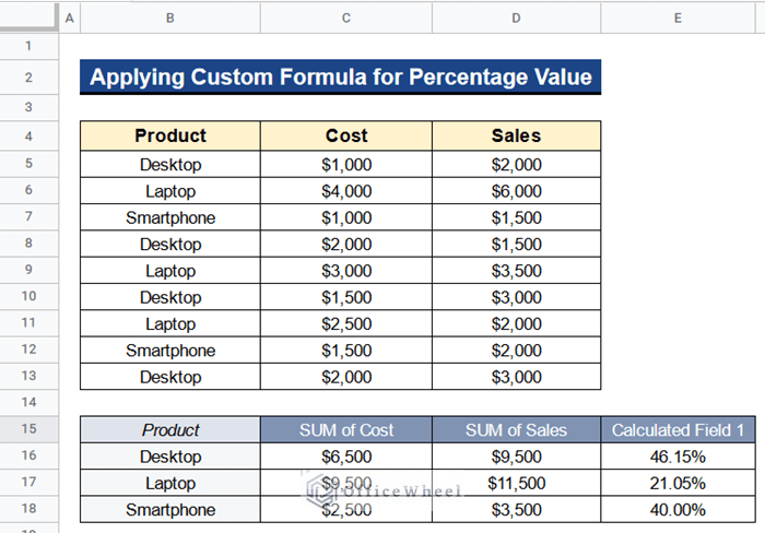
• Next, rename Cell E15 as Profit Percentage.
• In the end, Column E is showing the difference between the two columns, Columns C and D as the profit percentage of the products.

Read More: Calculate Percentage Difference Between Two Numbers in Google Sheets

Things to Remember

• Remember to untick the box beside Show Totals in the Rows menu under the Pivot Table Editor window because we don’t want the total values of the cost prices or sales prices of our dataset.
• Don’t forget to select SUM under the Summarize By menu in the Pivot Table Editor window during the calculation process. Otherwise, the result would be erroneous.

Conclusion

That’s all for now. Thank you for reading this article. In this article, I have discussed 2 suitable ways to find the difference between two columns in the Calculated Field of Google Sheets Pivot Table. Please comment in the comment section if you have any queries about this article. You will also find different articles related to google sheets on our officewheel.com. Visit the site and explore more.

Related Articles

• How to Find Missing Values Between Two Columns in Google Sheets
• Conditional Formatting Between Two Values in Google Sheets
• Use REGEXEXTRACT Function Between Two Characters in Google Sheets
• Generate Random Numbers or Text Between Limits in Google Sheets
• How to Find Correlation Between Two Columns in Google Sheets
• Google Sheets Count Cells Between Two Numbers with COUNTIF Function
• How to Use IF Condition Between Two Numbers in Google Sheets