Calculating the time between dates may be beneficial for company operations in a number of different circumstances. Project management is a good illustration of this. When assigning tasks to team members, you might need to determine how long it will take to complete them. The use of basic formulae in Google Sheets has made working with date and time simple. In Google Sheets, you can quickly determine how many days there are between two dates by either subtracting the dates (if you require all the days) or by utilizing formulae to determine if there are working or non-working days. In this article, I’ll demonstrate 6 simple ways to calculate the time between dates in Google Sheets. Here is an overview of what we will archive:
6 Simple Ways to Calculate Time Between Dates in Google Sheets
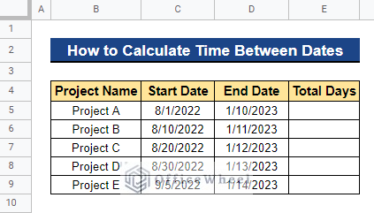
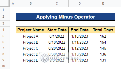
We will use the dataset below to demonstrate 6 simple ways to calculate the time between dates in Google Sheets. The dataset contains the project names as well as the start and end dates for each project. Now, we will determine how much time has passed between the projects’ start and end dates.
1. Applying Minus Operator
Dates are merely numbers with special formatting that makes them appear to date. Dates may be used in operations like addition and subtraction since they are integers. We can simply subtract two dates to get the time difference in Google Sheets.
Steps:
- Firstly, select the cell where you’re going to apply the formula. In our case, we selected Cell D5. Now, enter the formula below and press Enter–
=C5-B5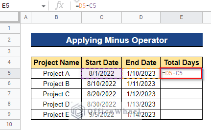
- Next, drag the Fill Handle icon downward to apply the formula to the remaining cells.
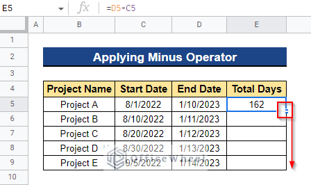
- As a result, you will get the total number of days between the two dates.
Read More: Calculate Number of Years Between Two Dates in Google Sheets
2. Merging MINUS and TODAY Functions
The MINUS function may be used to determine the time difference between two dates. It is identical to the first approach. The distinction is that we are utilizing a function rather than manually subtracting. Furthermore, it will exclude the commencement date from the calculation of the total number of days. In order to make the dataset more dynamic, we will utilize the MINUS function to determine the amount of time that has passed since a project’s Start Date. So here, we’ll use the TODAY function to get the time difference from the current date.
Steps:
- Select the cell to which you will be applying the formula first. In our instance, we decided on Cell D5. Enter the following formula now, then hit Enter–
=MINUS(TODAY(),B5)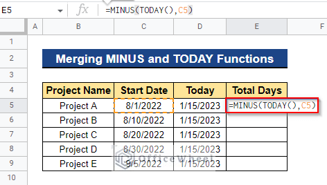
Formula Breakdown
- TODAY()
Here, the TODAY function provides a date value that represents the current date.
- MINUS(TODAY(),B5)
Then, the MINUS function determines the number of days passed from the Start Date to the current date.
- Next, to apply the formula to the remaining cells, slide the Fill Handle symbol downward.
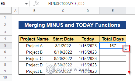
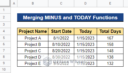
- As a result, you will get the total number of days that have passed since the project’s start date. Since we utilized the TODAY function, the total number of days will change daily.
Read More: How to SUMIF Between Two Dates in Google Sheets (3 Ways)
Similar Readings
- How to Link Cells Between Tabs in Google Sheets (2 Examples)
- Move Between Tabs in Google Sheets (3 Easy Ways)
- Google Sheets Count Cells Between Two Numbers with COUNTIF Function
- How to Use IF Condition Between Two Numbers in Google Sheets
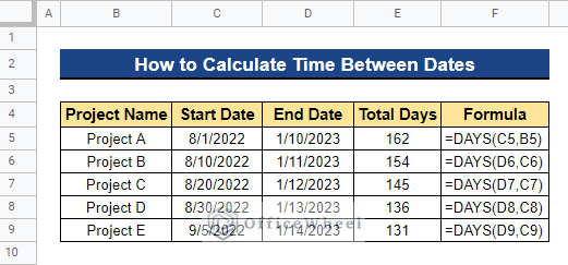
3. Employing DAYS Function
The total number of days between two dates may be determined in Google Sheets using the DAYS function. If you don’t care about eliminating weekends, holidays, etc., this is one of the simplest ways to compute the number of days between dates in Google Sheets.
Steps:
- First, choose the cell to which you will be applying the formula. In this instance, we chose Cell D5. Now, input the following formula and hit Enter–
=DAYS(C5,B5)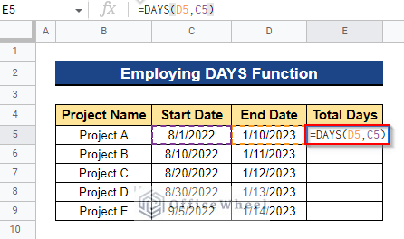
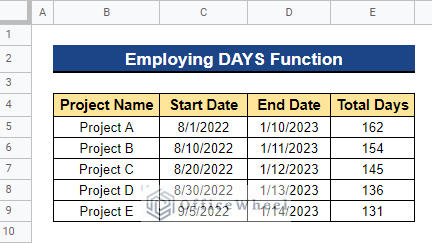
- Afterward, move the Fill Handle symbol downward to apply the formula to the remaining cells.
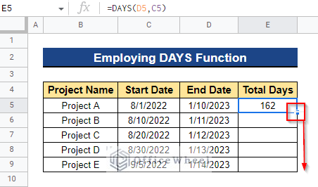
- You will thus receive the total number of days between the two dates.
Read More: How to Filter Between Two Dates in Google Sheets
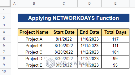
4. Applying NETWORKDAYS Function
Even while it’s convenient and simple to find the total number of days between two different dates, most of the time you simply need the number of working days instead. Although it’s not as simple as subtracting the data, figuring out how many working days there are between two different dates is not too difficult because Google Sheets includes a formula for it. The net working days between two different dates are provided by the NETWORKDAYS function. The number of working days is determined by considering both the start and finish dates. The weekends are thought to be occurring on Saturday and Sunday. Therefore, the days from Monday through Friday are all counted. Additionally, NETWORKDAYS can be modified to compute non-standard working weeks (i.e., not Monday through Friday) as well as to eliminate holidays.
Steps:
- Select the cell to which you will be applying the formula first. Here, we selected Cell D5. Type the following formula now and press Enter–
=NETWORKDAYS(B5,C5)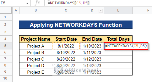
- Next, apply the formula to the remaining cells by dragging the Fill Handle icon downward.

- Thus, you will obtain the total number of working days between the two dates.
Similar Readings
- Generate Random Numbers or Text Between Limits in Google Sheets
- How to Find Correlation Between Two Columns in Google Sheets
- Insert Rows Between Other Rows in Google Sheets (4 Easy Ways)
- Find Difference Between Two Columns in Calculated Field of Google Sheets Pivot Table
- Difference Between COUNT and COUNTA in Google Sheets
5. Using DATEDIF Function
The definition of the DATEDIF function is Date Difference. It enables you to figure out how many days, months, or years there are between two dates. Like the DAYS function, the DATEDIF function operates in a similar way. The two key distinctions are that you use the start date first rather than the end date and that you must additionally specify a Unit for the syntax to determine how the difference will be reported. To calculate the time difference in days, months, and years, we may use units D, M, and Y, respectively.
Steps:
- Prior to applying the formula, pick the cell that it will go in. Here, Cell D5 was our selection. Now, insert the formula below and hit Enter. We use unit D here to display the time difference in days since we wanted to compute how many days there were between two dates.
=DATEDIF(B5,C5,"D")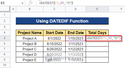
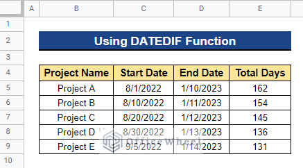
- By dragging the Fill Handle symbol downward, you can then apply the formula to the remaining cells.
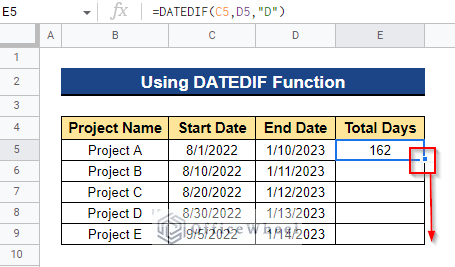
- Thus, it will display the total number of days between the two dates.
Read More: Find Number of Months Between Two Dates in Google Sheets
6. Combining TEXT and INT Functions
Occasionally we might desire to count the number of days and time that has passed between two dates in Google Sheets. Combining the TEXT and INT functions allows us to do this. The amount of time that has passed should be provided in the format of days, hours, minutes, and seconds.
Steps:
- Select the cell where you’ll apply the formula. We chose Cell D5 in this instance. Once you’ve entered the formula, press Enter–
=INT(C5-B5)&"d "&TEXT(C5-B5-INT(C5-B5),"HH:MM:SS")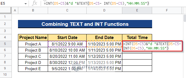
Formula Breakdown
- INT(C5-B5)
Here, the INT function rounds the total number of days passed to the nearest integer.
- TEXT(C5-B5-INT(C5-B5),”HH:MM:SS”)
The TEXT function converts the remaining time into the format HH:MM:SS.
- INT(C5-B5)&”d “&TEXT(C5-B5-INT(C5-B5),”HH:MM:SS”)
The output from the INT function and the TEXT function is combined using the & sign.
- After that, drag the Fill Handle indicator downward to apply the formula to the remaining cells.
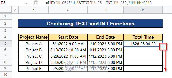
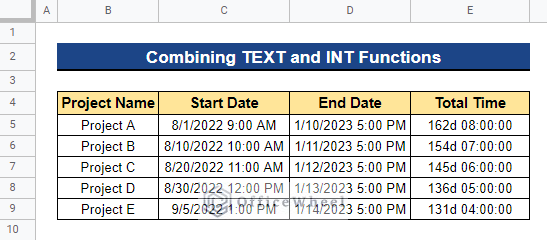
- As a result, you will get the total amount of time that has passed in the format of days, hours, minutes, and seconds.
Read More: How to Calculate Hours Between Two Times in Google Sheets
Conclusion
It ends here. I’m grateful that you patiently read this article. I’m hoping that this will make it easier for you to determine in Google Sheets how much time has passed between the two dates. In the comment section below, please feel free to post any questions or suggestions. Visit our website Officewheel.com; if you’re interested in reading more of this creative writing on Google Sheets.
Related Articles
- How to Find Missing Values Between Two Columns in Google Sheets
- Conditional Formatting Between Two Values in Google Sheets
- How to Insert Lines Between Cells in Google Sheets
- Use REGEXEXTRACT Function Between Two Characters in Google Sheets
- How to Find Unique Values Between 2 Columns in Google Sheets
- Calculate Percentage Difference Between Two Numbers in Google Sheets
- How to Remove Spaces Between Words in Google Sheets