One of the most widely used management tools for calculation and documentation is Google Sheets. However, the dataset frequently contains repeated values, which add complexity and redundancy to the data. Thus, being able to merge duplicate rows in Google Sheets is a crucial ability.
A Sample of Practice Spreadsheet
5 Methods to Merge Duplicate Rows in Google Sheets
There are five options available in Google Sheets to merge duplicate rows based on the circumstance and the data. Each with a special benefit and drawback of its own. We have used practical examples for a better understanding of the methods.
1. Applying the Data Clean-Up Option
One of the most simple methods to merge duplicate rows is to use the Data Clean-Up tool. Simple in its form. We are going to demonstrate it with a practical example.
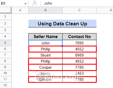
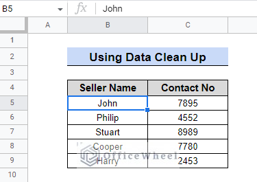
Assume a corporation has a database with the names of its sellers and their phone numbers. It is, nevertheless, filled with several duplicates. We will thus create a clean and organized dataset.
Here are the steps:
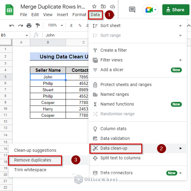
- Data > Data Clean-up > Remove Duplicates
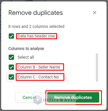
- Check “✓” the boxes under the Columns to analyze section. (If there is a header, mark “✓” in the Data has header row)
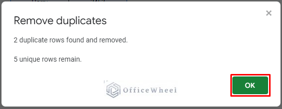
- A small window will pop up describing the result. Click OK.
- Finally, the result will appear. It deleted the Duplicates values and showed only the unique values.
2. Using UNIQUE, FILTER & JOIN Functions
It is a two-way process. Simple and brief in style. The UNIQUE function will be used initially, followed by the JOIN function and the FILTER function. In contrast to the prior method, this one allows you to calculate or add duplicate values. Below is a step-by-step explanation of the procedure with an actual example.
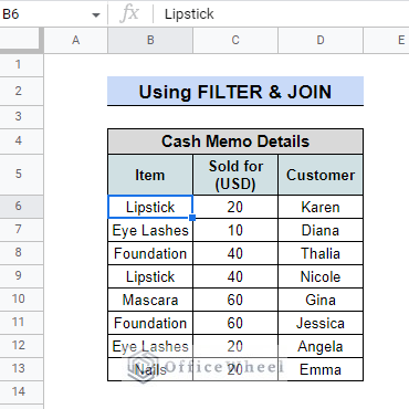
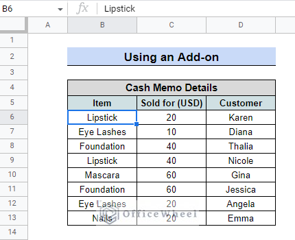
You will discover a table containing information taken from a cash memo for a cosmetics store. What kind of product was sold, how much did it cost, and to whom. By merging the duplicate values, we will sum up the entire table.
Steps:
- Create a new table on the side of the worksheet with the same title and structure.
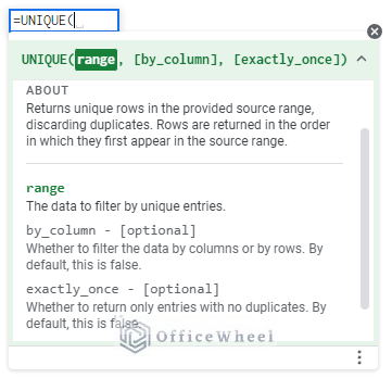
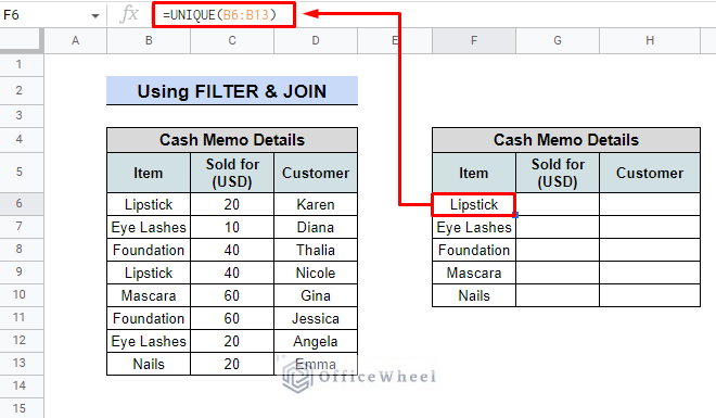
- Use the UNIQUE function to bring out unique products. We are going to use the following formula.
=UNIQUE(B6:B13)As a result, as seen in the above image, it will list the unique products in the Item column.
- Now we are going to use the JOIN function in order to merge the rows.
- By looking for equal and matching values in column B, the FILTER function will assist in identifying the relevant and logical rows.
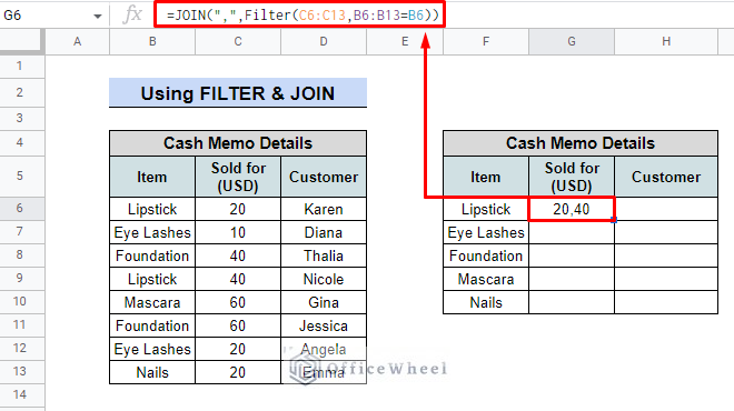
- We will use the following formula in cell G6.
=JOIN(“,”,FILTER(C6:C13,B6:B13=B6))As you can see, Lipstick was offered for 20 and 40 USD each time it was sold. A comma (,) separates the sold prices from the duplicate rows after they were combined.
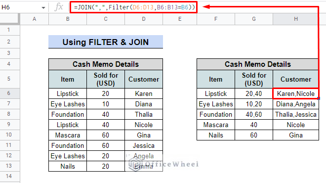
- We are going to use the same formula to fill the Customer Column. The formula is:
=JOIN(“,”,FILTER(D6:D13,B6:B13=B6))Similar to before, it combined the cells and used commas to separate the Customer names.
Read More: How to Filter with Custom Formula in a Pivot Table of Google Sheets
3. QUERY Function to Merge Duplicate Rows
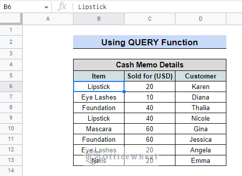
The most robust and flexible feature of Google Sheets is the QUERY function. Although it has many features, we need a formula that can locate the duplicate values and merge the cells in the context of merging duplicate rows. Additionally, in this example, we’ll use the same dataset.
Steps:
- We’re going to start by creating a table header that resembles the dataset.
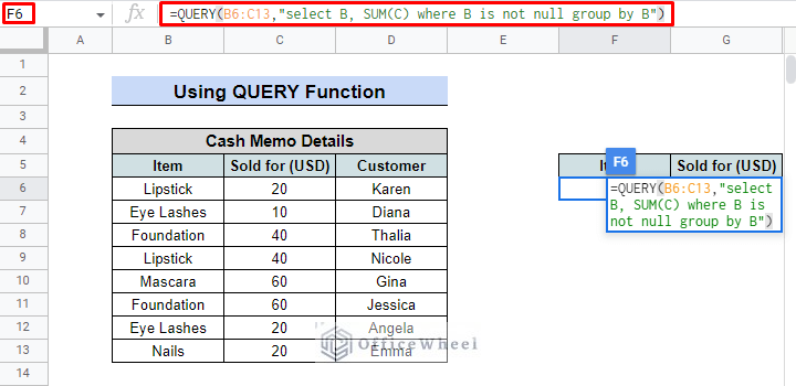
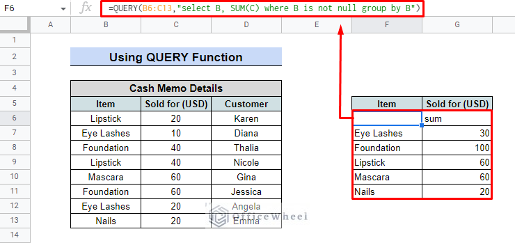
- We will employ the QUERY function and the subsequent method in cell F6, which is located beneath the Item header.
=QUERY(B6:C13, "select B, Sum(C) where B is not null group by B")The formula will produce the intended result, a table, below cell F6.
Similar Articles
- How to Refresh a Pivot Table in Google Sheets (3 Ways)
- Google Sheets: Create a Pivot Table with Data from Multiple Sheets
- How to Group by Month in a Google Sheets Pivot Table (An Easy Guide)
- How to Apply and Work with a Calculated Field of a Google Sheets Pivot Table
- How to Sort a Pivot Table in Google Sheets (An Easy Guide)
4. Using the Pivot Table to Merge Duplicate Rows
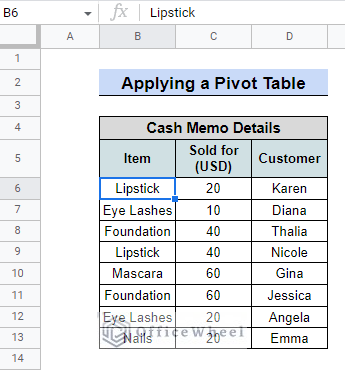
Using a Pivot Table is another technique to merge duplicate rows in Google Sheets. The advantage of employing a pivot table is that it can compute values and derive summations. Below is a description of the entire procedure with an appropriate example. The dataset that we previously used will be used again.
Steps:
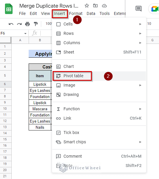
- Insert > Pivot Table
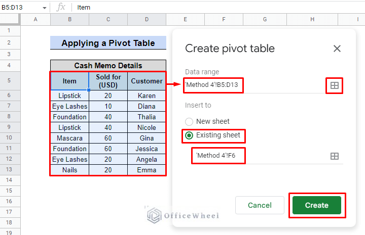
- A popup titled “Create Pivot Table” will appear. Here, we must define the data range and cell number where the table will be created.
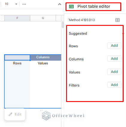
- Thus, As seen in the figure, a column with the title Pivot Table Editor will appear on the right side of the Google sheet, and a table will appear in the specified cell. Namely, in cell F6.
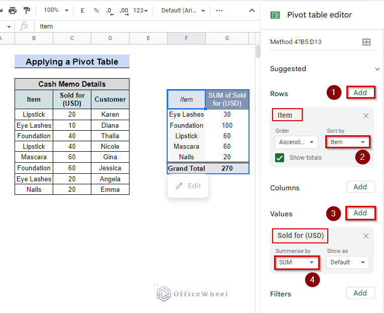
- The editor includes a lot of user-friendly functions. However, we will only use Rows and Values for this example. So, Row > Add > Sort by > Items
- Don’t forget to Check the Show totals box
- Values > Add > Summarize by > SUM
The table as it is depicted in the above image will then be found. In addition to combining duplicates, it also summed the entire sales price. The advantage of the Pivot table over other techniques is simple to understand.
Read More: Apply a Pivot Table Slicer in Google Sheets (An Easy Guide)
5. Make Use of Add-Ons
In Google Sheets, there are really two add-on options for combining duplicate values. The Remove Duplicates tool is one, while the Power Tool is the other. Make sure you obtain the add-ons from Google Workspace Marketplace before attempting to utilize them (They are free to use). We’ll use the same dataset as before to show how the add-ons can be used.
5.1 The Remove Duplicate Add-On
There are 5 tools included in this add-on for eliminating duplicates in Google Sheets. In order to merge duplicate rows, we will use the following steps.
Steps:
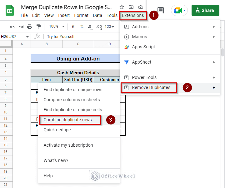
Navigate the tool from Extensions > Remove Duplicates > Combine Duplicate Rows
A window will pop up. Here, we have to perform a few steps:
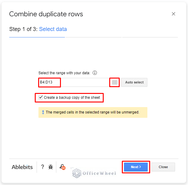
- Select the data range. For this example it’s B4:D13. If you want to keep a copy of the original data check “✓” the create a backup copy of the sheet.
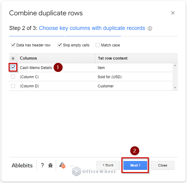
- In step 2 of the box, select the columns that have duplicate values. For this example, it’s the Item column. Then click Next.
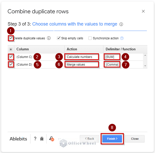
- We will decide how the values of the duplicate cells will merge in the third step of the process.
- We have two columns: one contains summable numerical values, and the other contains customer names.
- The names can be combined with a comma.
- We can adjust the desired parameter by navigating the Column, Action, and Delimiter/function columns of the box, as shown in the image below.
Here, the numbers in the image above represent the option clicks you have to perform.
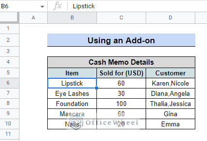
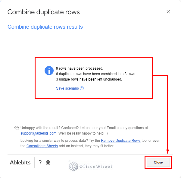
- After clicking the Finish button, a window will pop up with the result details. Click the Close button to see the table.
5.2 The Power Tool Add-On
There are more than 30 intelligent features in Power Tools that Google Sheets lacks the most. For this case, check the steps below.
Steps:
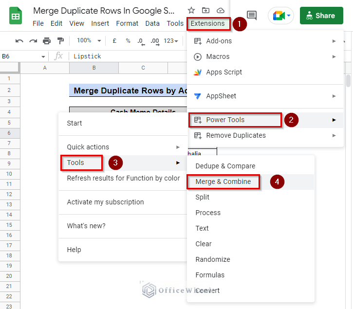
- Navigate the tool from Extensions > Power Tools > Tools > Merge & Combine
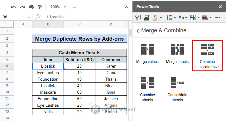
A tab named power tools on the right-hand side will appear.
- Select Combine Duplicate Rows
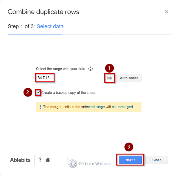
- The exact three-step window will appear as before. Here, you must choose the data range. In this instance, it is B4:D13. If you want to preserve a copy of the original data, make a backup copy of the sheet. Then click Next.
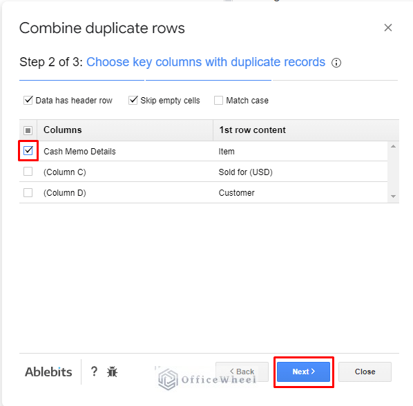
- Pick the columns with duplicate values in step 2 of the box. The Item column in this instance then presses Next.
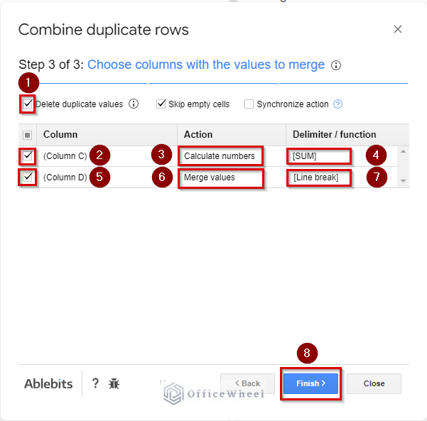
- In the third step of the process, we will choose how the values of the duplicate cells will merge. This time slightly different from the earlier approach. The required option clicks are shown as numbers in the image above.
- Mark “✓” to Delete the duplicate values.
- Column > “✓” (Column C) > Action > Calculate Numbers > Delimiter > SUM
- Column > “✓” (Column D) > Action > Merge Values > Delimiter > Line Break
- Click Finish to finalize.
- A window displaying the results will appear. Click Close.
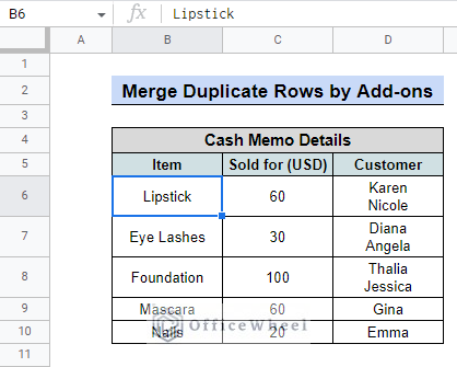
The table will then appear as directed. The duplicate rows have been combined, the Sold values have been added, and the Customer names are now displayed with a line break.
Conclusion
You can now either merge the duplicate values in rows or total them in Google Sheets, depending on your objective. The only thing you need to know is which feature of Google Sheets will best serve your needs. You can visit our website, OfficeWheel, for further details.
Related Articles
- How to Use a Custom Formula in a Google Sheets Slicer (An Easy Guide)
- Google Sheets Slicer Tutorial
- Find the Top 10 Values in a Google Sheets Pivot Table (2 Easy Examples)
- Google Sheets Pivot Table: Calculate the Percentage of Total (2 Easy Examples)
- Google Sheets Pivot Table: How to Remove Grand Total or Subtotal
- Group Dates in a Google Sheets Pivot Table (An Easy Guide)
- How to Make a Pivot Table in Google Sheets (A Comprehensive Guide)
- Pivot Table Formatting in Google Sheets (3 Easy Ways)

