Google Sheets Pivot Table: Calculate the Percentage of Total (2 Easy Examples)

Percentage calculations are crucial when analyzing data. They give a clearer view of the distribution of values. We can make things even easier by taking advantage of the pivot table. In this article, we will look at how to find the percentage distribution of the total in a Google Sheets pivot table step by step.

Let’s get started.

2 Examples of How to Calculate the Percentage of Total in a Google Sheets Pivot Table

1. Find the Percentage of Grand Total or Subtotal in a Google Sheets Pivot Table

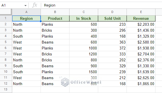
For our example, we will use the following dataset:

Using this dataset, we have created a simple pivot table:

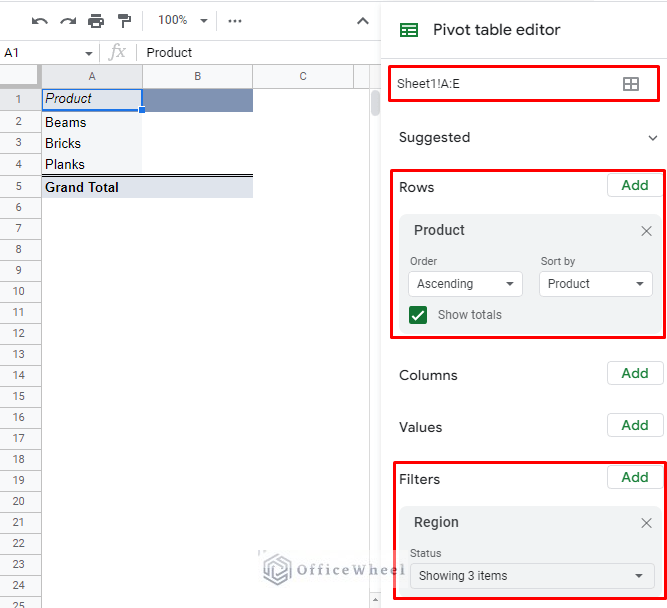
Note: We have filtered out the blank cells using the Filters panel.

The purpose of this pivot table is to show the percentage distribution of Revenue for each Product.

Step 1: To the existing pivot table, add Revenue to the Values panel.

Values > Add > Revenue

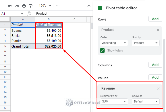
This column shows the distribution of revenues for each product, as well as the Grand Total of the Revenue column.

Step 2: Add another Revenue field in the Values panel. But this time, click on the ‘Show as’ drop-down to bring out all the options.

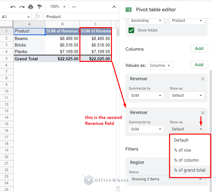
Step 3: Click on the ‘% of grand total’ option to present the second Revenue field as the percentage distribution of revenue for each Product.

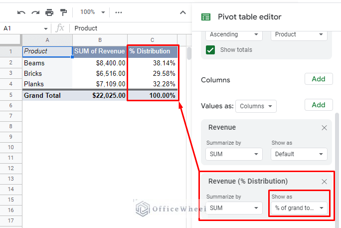
Thanks to the Pivot table editor, we have calculated the percentage distribution of the Grand Total of Revenue in a Google Sheets pivot table in just 3 steps. And that with no complicated formulas involved!

2. Find the Percentage Sold or Unsold from the Total in a Google Sheets Pivot Table

In our following example, we will look at percentage differences. To be more precise, we will try to find the percentage of the sold and unsold products from the total.

However, these fields cannot be directly inputted and require a formula. And the best way to insert a column with a formula in a Google Sheets pivot table is to use a Calculated Field.

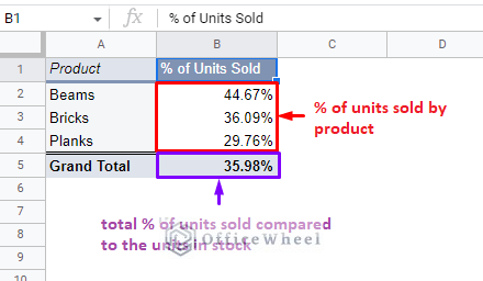
I. Calculate the Percentage of Sold Units from the Total Units In Stock

Step 1: Create a new Calculated Field. Rename it to ‘% of Units Sold’.

Values > Add > Calculated Field

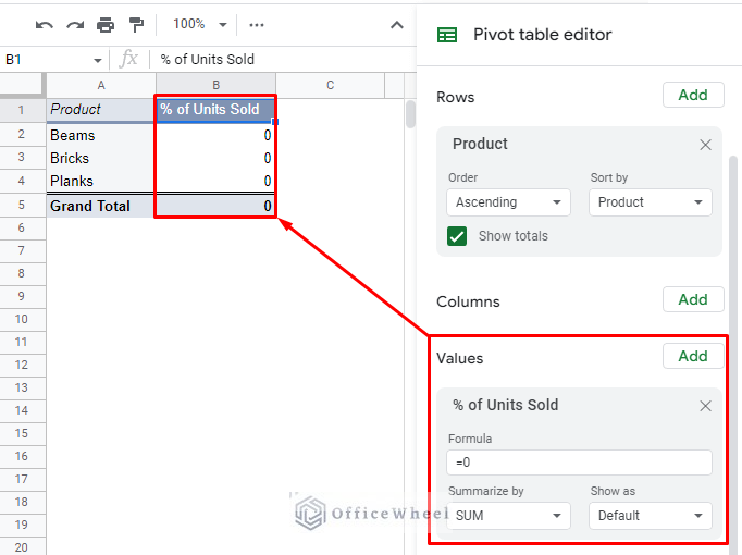
Step 2: Apply the following formula to calculate the percentage of units sold:

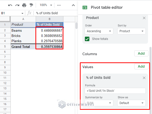
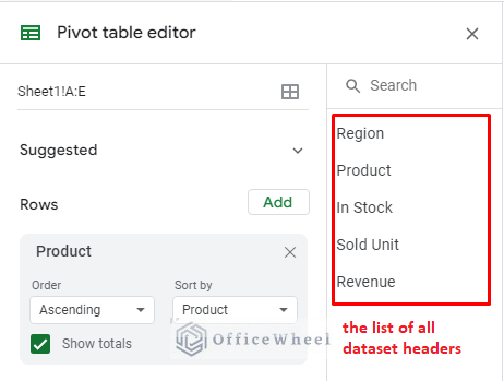
Remember that pivot tables use the names of the table headers of the source dataset in formulas instead of data ranges.

Tip: You can find the list of all headers on the right-side of the Pivot table editor.

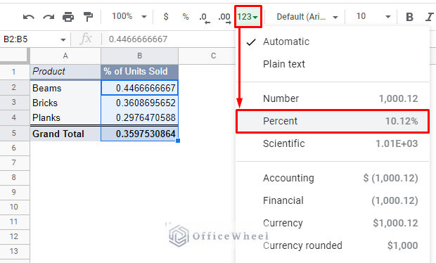
Step 3: Format the values to percentages from the Toolbar.

The result:

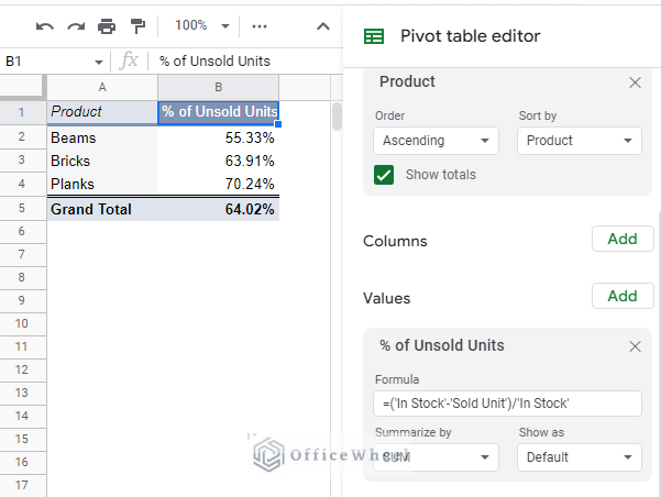
II. Calculate the Percentage of Unsold Units from the Total

This example follows similar steps as the previous one. The only difference is in the name and formula.

Step 1: Create a new calculated field and name it ‘% of Unsold Units’.

Values > Add > Calculated field

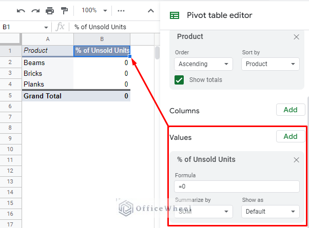
Step 2: Enter the following formula to calculate the percentage of unsold units.

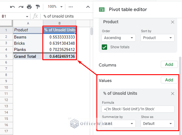
Step 3: Format the values to show percentages.

Final Words

That concludes how we can calculate the percentage of the total in a Google Sheets pivot table. The two examples are the most common uses, especially in calculating the percentage of the grand total or subtotal.

Thanks to the picot table editor, we don’t have to go through the hassle of creating a separate column to accommodate a complex formula.

Feel free to leave any queries or advice you might have in the comments section below.

Related Articles for Reading

• Google Sheets: Create a Pivot Table with Data from Multiple Sheets
• Using Custom Formula in a Google Sheets Pivot Table (3 Easy Ways)
• How to Group by Month in a Google Sheets Pivot Table (An Easy Guide)
• How to Filter with Custom Formula in a Pivot Table of Google Sheets
• Pivot Table Formatting in Google Sheets (3 Easy Ways)