In this simple tutorial, we will look at how we can apply and utilize a Calculated Field in a Pivot Table of Google Sheets.
Let’s get started.
What is the ‘Calculated Field’ in a Pivot Table?
We all know that the pivot table is a great tool to summarize data. This is mostly thanks to the built-in metrics that are available for all users to easily use. These include sum, average, variance, median, etc.
However, these are only the basic calculations that are most commonly used. But what about the ones that are not?
That is where the Calculated Field comes in.
The calculated field allows users to create their own formulas to perform calculations that are not built-in Google Sheets Pivot Table.
These custom formulas take data from the source table, perform the calculations according to the formula and output them in a column of a pivot table.
This is useful especially when you want to include a calculation in a pivot table but do not want to change the source dataset.
How to Add and Use a Calculated Field in a Pivot Table of Google Sheets
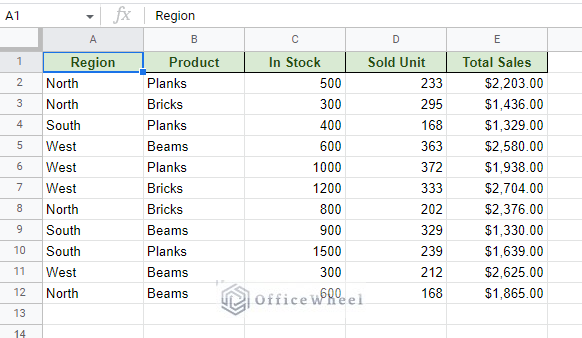
To show the process, we will use the following dataset as the source for the pivot table:
Now to create the pivot table:
- Select the entire columns (A to E) to add to the pivot table
- Click Insert > Pivot Table. The insert tab is on the top of the window.
- Select New Sheet when prompted to create the pivot table in a new worksheet.
For this example, we have used Product as the primary column value.
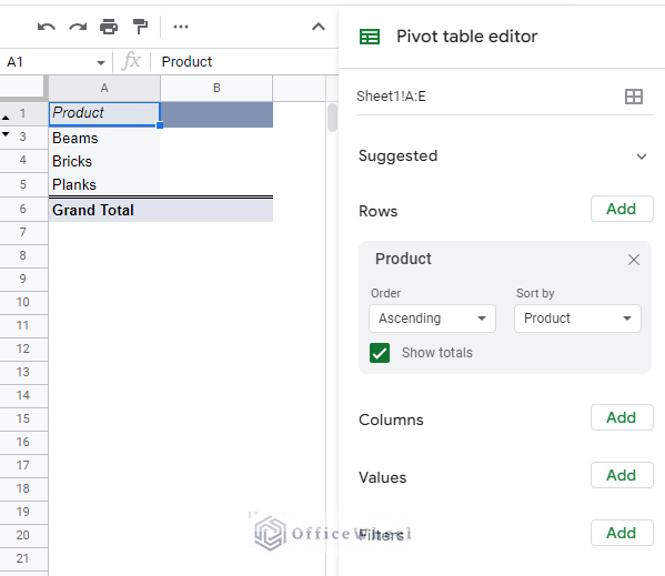
Note: Hide row 2 to ignore the blank cells of the source dataset.
Let’s say we want to add a column that shows us the unsold number of products in each category.
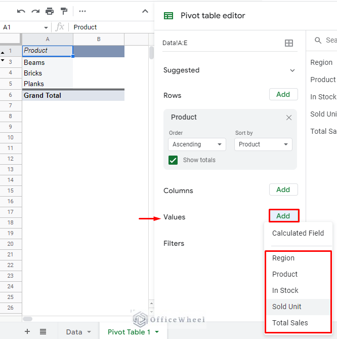
Normally, we’d go to the Values section to add a column. But as you can see, the columns that we can add, or eventually filter, do not meet our objective.
We must create a separate column to include our calculation there, a.k.a. a calculated field.
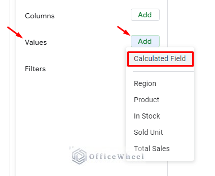
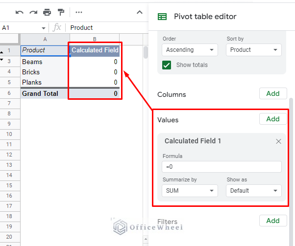
Step 1: Add a Calculated Field from the Values section.
Values > Add > Calculated Field
This will place a default Calculated Field column in the pivot table:
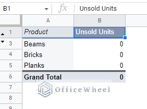
Step 2: Rename the calculated field.
Step 3: In the formula panel, add the following formula to calculate the number of unsold units. This is essentially the difference between ‘In Stock’ and ‘Sold Unit’ values.
='In Stock'-'Sold Unit'This formula subtracts the values in each row of the columns from the source dataset.
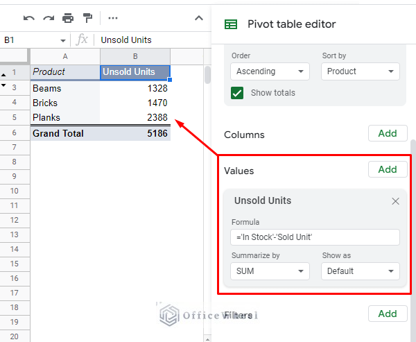
And we are done!
But what we’ve just shown is a simple calculation. The Calculated Field in the Google Sheets pivot table can do much more. Let’s look at a few more examples from the same source dataset:
- Add a 5% VAT to the Total Sale price.
- Calculate the percentage of the units sold.
- Calculate the max number of units sold for each category.
1. Add VAT to Total Sales Price in a Pivot Table using a Calculated Field
Let’s add another calculated field for this example. Simply click on the Add button in the Values section:
Values > Add > Calculated Field
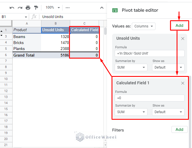
A second calculated field will be added to the existing pivot table.
Let’s rename this as ‘Sales with VAT (5%)’. Then add the following custom formula:
='Total Sales'+((5/100)*'Total Sales')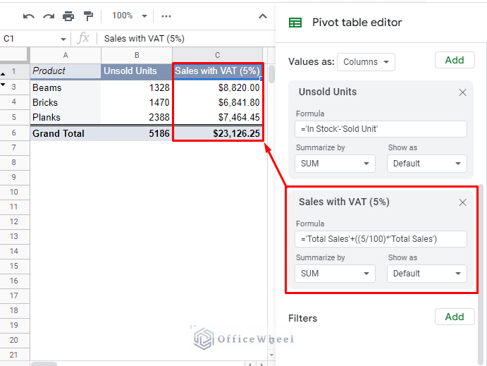
2. Calculate the Percentage of Units Sold in a Pivot Table of Google Sheets
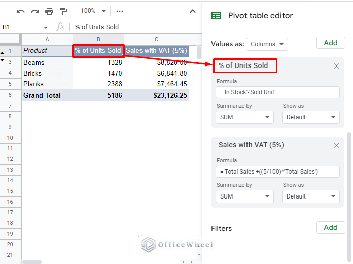
Just for this example, let’s replace the Unsold Units calculated field with the percentage of units sold.
Step 1: Update the column header to ‘% of Units Sold’. This update will also change the name in the Values section.
Step 2: Update the formula to:
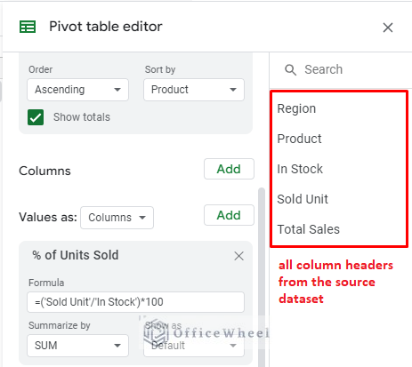
=('Sold Unit'/'In Stock')*100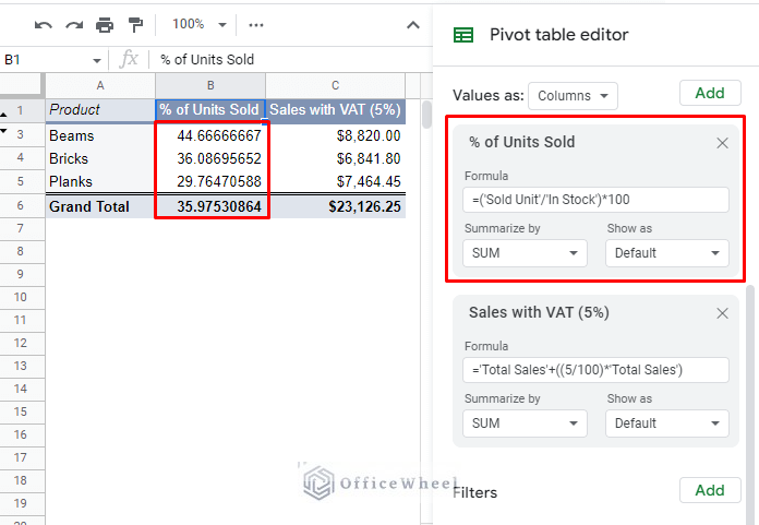
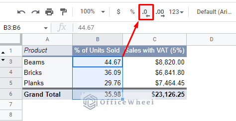
Step 3: Format the pivot table to show the percentage values in 2 decimal places. Simply use the drop-down menu from the Toolbar.
3. Add a Custom Summarized Calculated Field (Max Units Sold)
So far, all of the outputs have been a sum of conditions applied by the formula in the calculated field. But now, we want to find the maximum number of units of each individual product sold (not the SUM).
Step 1: We start the same way by adding a calculated field from the Values section and naming it ‘Max Units Sold’.
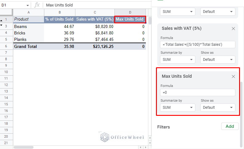
Step 2: Input the formula:
=MAX('Sold Unit')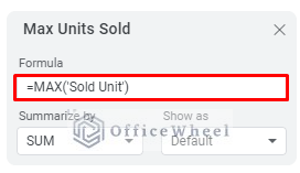
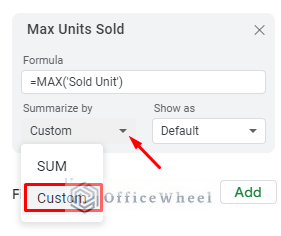
Usually, this is the step where we get the results, but not this time.
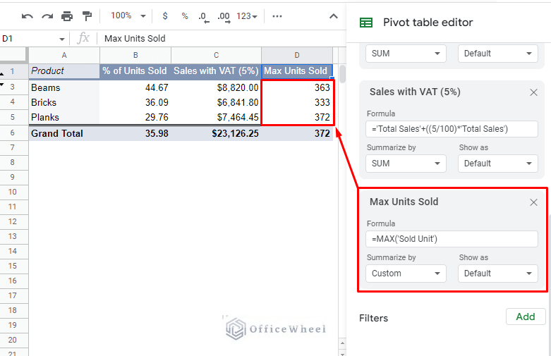
Step 3: Show the proper results of the maximum, we must update the Summarize by option from SUM to Custom.
The result:
Points to Note about Calculated Fields
The primary purpose of calculated fields is to provide more flexibility to perform calculations in the pivot table of Google Sheets. However, it is not a perfect solution.
- Calculated fields can only reference columns. You cannot reference individual cells in the worksheet.
- Data can only be referenced from the source dataset. You cannot reference data from the pivot table.
- Calculated fields only use column headers from the source dataset as reference. You must make sure that the names are correctly input and are within single quotes (‘’). Tip: All the column header names are listed on the right side of the Pivot table editor.
Final Words
Calculated fields are a great way to customize and bring a new layer of data to a pivot table of Google Sheets. As we have seen in this article, the calculated fields can also show the results summarized by SUM and also custom.
Feel free to leave any queries or advice you might have in the comments section below.
Related Articles for Reading
- How to Filter with Custom Formula in a Pivot Table of Google Sheets
- How to Sort a Pivot Table in Google Sheets (An Easy Guide)
- Using Custom Formula in a Google Sheets Pivot Table (3 Easy Ways)
- How to Refresh a Pivot Table in Google Sheets (3 Ways)
- Google Sheets Pivot Table: Calculate the Percentage of Total (2 Easy Examples)