Google Sheets: Create a Pivot Table with Data from Multiple Sheets

A pivot table is a powerful data summarization tool for any spreadsheet. Since it’s a spreadsheet, it is not uncommon to have data coming from multiple worksheets. So, a question comes to mind: Can you create a pivot table using data from multiple worksheets in Google Sheets?

Yes and No.

Confusing right?

In this simple guide, we will show you exactly why you can’t directly create a pivot table from multiple sheets, but also show you how we can actually do so by using tools and functions available in the spreadsheet application.

Let’s get started.

How to Create a Pivot Table using Multiple Sheets in Google Sheets

We mentioned that it is not directly possible to create a pivot table from multiple sheets. And here’s why:

The emphasis is on the word ‘directly’, since the Pivot Table Editor does not allow the user to input multiple ranges at once.

Here we tried to add the data ranges from two separate worksheets in the spreadsheet to create a pivot table. But as you can see, multiple ranges are not accepted. This restricts us from creating a pivot table with data from multiple sources.

However, we can overcome this issue with a simple solution: extract the data from multiple sources into a single worksheet and create a pivot table from this worksheet.

Let’s see how it’s done step by step:

Step 1: Validate the Source Datasets

The first thing we must do is check whether the source datasets are valid or not. By that, we mostly mean whether the headers of all the datasets match or not.

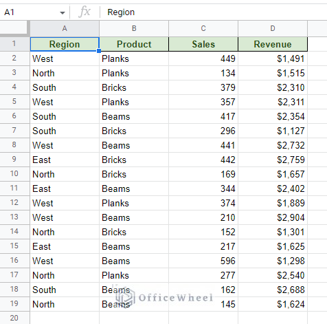
For example, here we have the first dataset:

And the second dataset that we will use to create the pivot table:

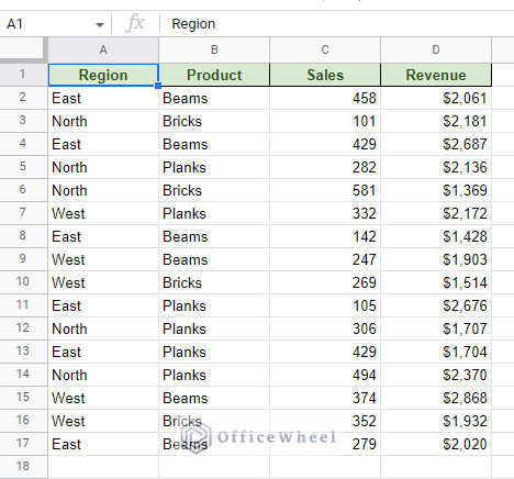
As you can see, the layouts and headers of both worksheets are exactly the same, the only thing that differs is the data in them.

This is an ideal situation that will make combining these datasets easy.

Step 2: Consolidate/Combine the Datasets

This is the most important step of the entire process: the consolidation of data from the different sources. And we have two ways to go about it.

Given that the datasets have valid headers and data for the pivot table, we can:

1. Use a simple reference array to extract all the data to a single worksheet.
2. Use a QUERY formula to extract all the data to a single worksheet.

Option 1: Using Regular Cell Reference to Retrieve the Data as an Array

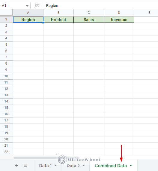
Step 1: Create a new worksheet to hold the data. Add headers to match the datasets.

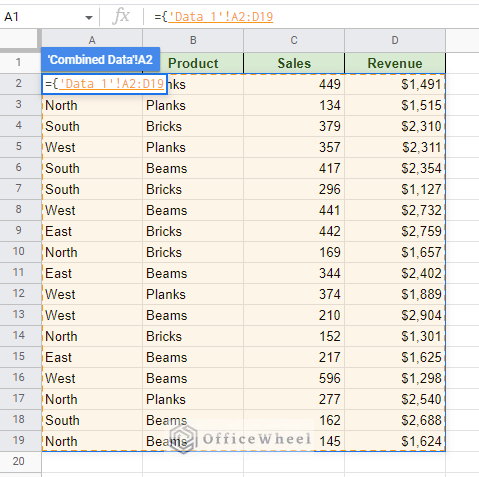
Step 2: Open a formula in cell A2 and open curly braces.

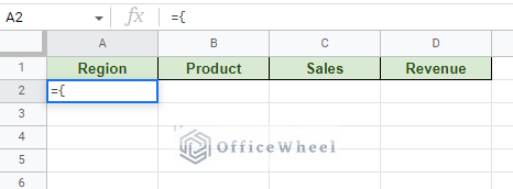
The curly braces will hold the array of cell references from the different worksheets.

Step 3: Put the cursor within the curly braces and go to the different worksheets to select the range.

For Data 1 worksheet:

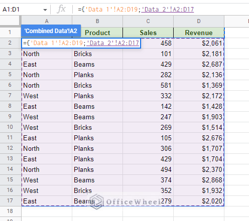
Input a semicolon (;) to separate the ranges and select the data from Data 2 worksheet:

Step 4: Close the curly brace and press ENTER.

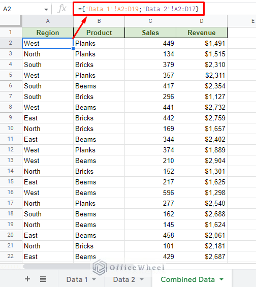
We can now move to create a pivot table with this Combined Data worksheet.

Option 2: Using QUERY Function (Recommended)

This next option is to simply enclose the array used in Option 1 inside a function. Namely the QUERY function.

Step 1: Create a new worksheet where you will put the combined data. Add the headers that are required.

Step 2: Open the QUERY function in cell A2 and open a curly brace after.

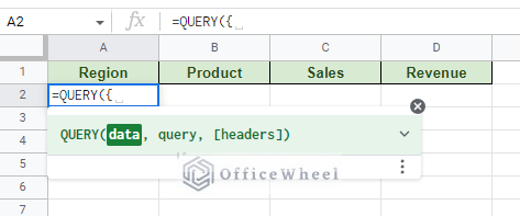
Step 3: Go to each dataset and add the range of values. Separate each range with a semicolon (;).

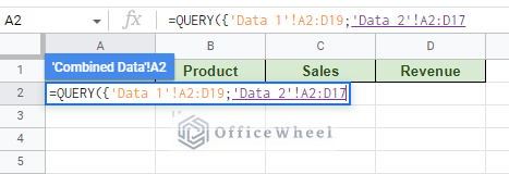
Step 4: Close the curly brace and parentheses and press ENTER.

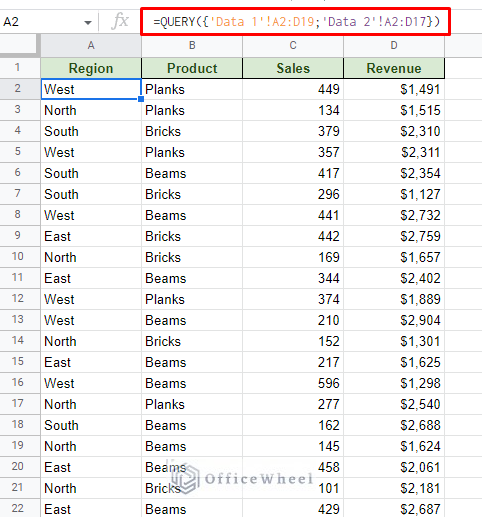
Alternatively, if you want to make this extraction of data dynamic and include any new entry done to any source dataset, make these two changes:

1. Remove the cell range limits (A2:D19 to A2:D and so on)
2. Enclose the array within a SORT function. This will help push all the blank cells in the range downward.

This will sort the source data but will have no impact on the eventual pivot table.

You can now create a pivot table with this combined data.

Step 3: Create the Pivot Table

All that is left to do is to create a pivot table from the dataset that we have just created.

If you already know how then that’s great, you are done. If not, follow these simple steps:

Step 1: Select entire columns of the data. Click on the worksheet column headers (A, B, C…) to select the entire column.

Step 2: Navigate to Pivot Tables from the Insert tab.

Insert > Pivot Tables

Step 3: Select where you want the pivot table to appear. The same worksheet or a new one.

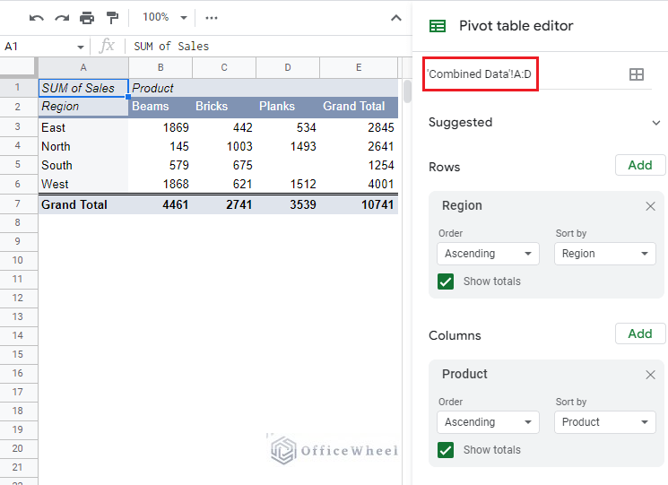
Here is an example pivot table using the combined data of multiple worksheets in Google Sheets:

Learn More: How to Make a Pivot Table in Google Sheets (A Comprehensive Guide)

Final Words

That concludes our step-by-step guide on how we can create a pivot table using data from multiple sheets in Google Sheets.

While a direct method would have been handy, Google Sheets provides its users with enough tools to take a longer, yet simpler, approach to this issue.

Feel free to leave any queries or advice you might have for us in the comments section below.

Related Articles for Reading

• Using Custom Formula in a Google Sheets Pivot Table (3 Easy Ways)
• Group Dates in a Google Sheets Pivot Table (An Easy Guide)
• How to Apply and Work with a Calculated Field of a Google Sheets Pivot Table
• How to Filter with Custom Formula in a Pivot Table of Google Sheets
• Pivot Table Formatting in Google Sheets (3 Easy Ways)