In this article, we will go through a comprehensive tutorial on Google Sheets Slicer. We will discuss how to apply and use a slicer in Google Sheets with some essential tips to go along with it.
Let’s get started.
What is a Google Sheets Slicer?
The Slicer is essentially a visual filter for the spreadsheet application. Some features of the slicer are:
- You can apply multiple slicers to a single dataset. This is essentially filtering with multiple conditions.
- Slicers can be customized to be color-coded to help distinguish between different filters.
- The dataset state is not changed when filtering with a slicer.
Fun Fact: The name “slicer” comes from the fact that the tool slices data into more understandable pieces.
How-To Tutorial for Slicer in Google Sheets
For this tutorial, we will use the following worksheet:
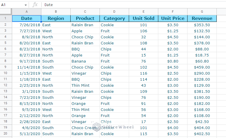
This dataset has 50 rows of data. While we can apply a slicer right here, using a filter would be more intuitive.
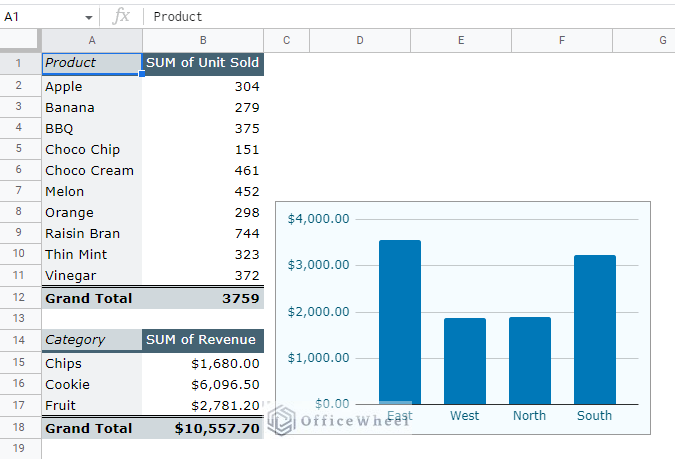
A slicer is best used alongside pivot tables.
Since the tool is a visual filter, using it on a dashboard with charts and pivot tables provides a quick and easy way to present the data more clearly.
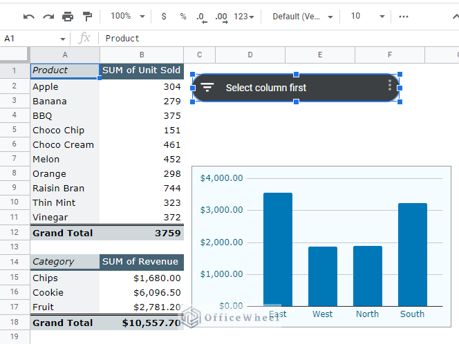
As such, we have used the dataset above to create a simple dashboard containing pivot tables and a chart:
Learn More: How to Make a Pivot Table in Google Sheets (A Comprehensive Guide)
Now, let’s add and use a slicer for this dashboard.
How to Insert a Slicer in Google Sheets
Step 1: To insert a slicer, we must first select the cells that will be the data range of the slicer.
To do that, we can select the cells of the source dataset. Which in this case is in Sheet 1
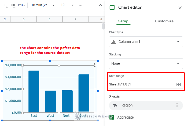
Or we can take a more intuitive approach.
You see, the different elements of the dashboard (the pivot tables and the chart) already stem from the source dataset. So, we can simply select one of these elements, in this case, the chart, to give us the data range for the slicer.
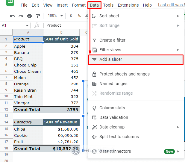
Step 2: Navigate to the Data tab and select the ‘Add a slicer’ option.
Data > Add a slicer
Step 3: The slicer should now appear in the middle of the worksheet. Since the slicer is independent of cells, you can simply click and drag it to a suitable position.
Set Up Data Conditions for a Slicer
Once we insert the slicer, the first thing we have to do is select the column or primary data which we will filter the dashboard by. Usually, this is immediately prompted by Google Sheets when inserting a slicer.
To do this, we open the slicer menu. Simply click on the slicer to bring it out. The first and primary tab that is presented to us is the Data tab. It is here we will set the primary conditions, data range and column condition, for the slicer.
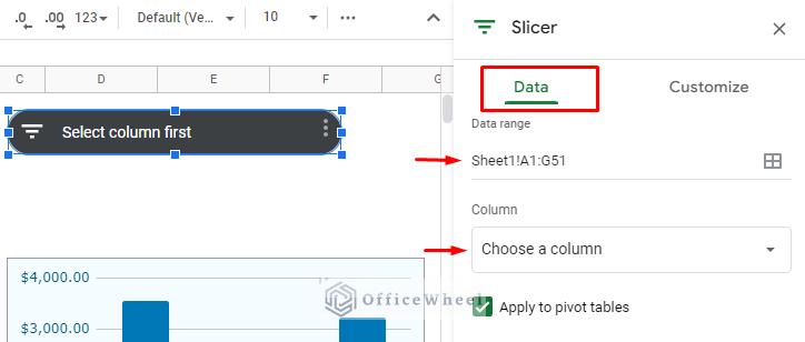
Clicking on the Column drop-down will present us with all the column options that we can filter the dashboard by. That is, as long as the data range that was selected is correct.
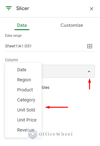
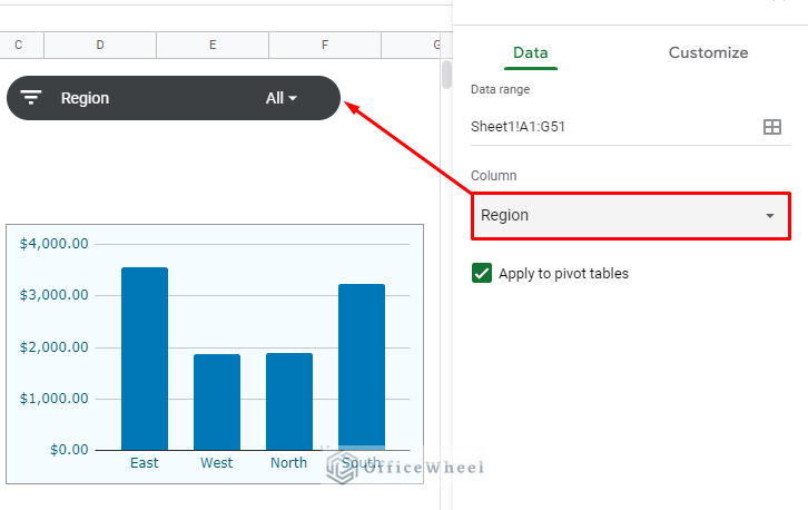
We want our data to filter by the regions and thus we select Region as the column option.
Customize the Slicer Appearance
In a dashboard, it is always a good idea to make your slicer stand out or follow the current theme of the spreadsheet.
For that, we have the Customize tab to work within the Slicer menu.
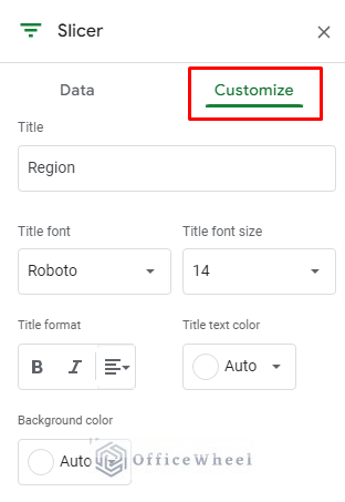
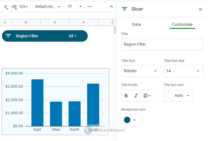
As you can see, you can set the Title of the slicer as well as customize the font. You can even set the font and background color of the slicer.
Here is what our slicer looks like with some customization:
Add Multiple Slicers in Google Sheets
One of the biggest advantages of using slicers in Google Sheets is that you can add multiple of them.
This means that you can have a dashboard that has multiple layers of filters each with different conditions!
To add a new slicer, simply follow the same step you have used to insert the first slicer.
Select the data range > Data tab > Add a slicer

For this Google Sheets slicer tutorial, we have set the second slicer to filter the dashboard by Date. We have also added a few customizations.
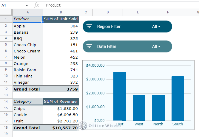
That concludes the part of inserting a slicer in Google Sheets. Next, we will look at how to work with these newly inserted slicers.
How to Filter Data Using a Slicer
Filtering with slicers is no different from using regular filters in Google Sheets. Even the filter menu interface for both tools is similar. This adds a lot of points to the user-friendliness of the application.
To open the filter menu of the slicer, simply click on the filter icon on the left-hand side:
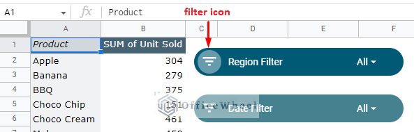
The filter menu:
Here you can see that we have two ways to apply a filter using a slicer:
- Filter by value (opened by default)
- Filter by condition
We will show you how to work with both options using examples.
1. Filter by Value (Filter Regional Data in Google Sheets)
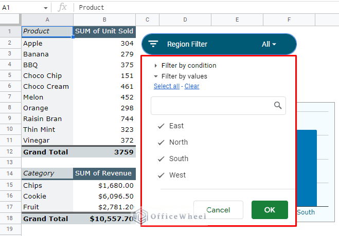
The ‘Filter by value’ option is open by default. Here, all the unique options in the column are listed and checked.
To filter by the listed values, simply check the values that you want and uncheck the others.
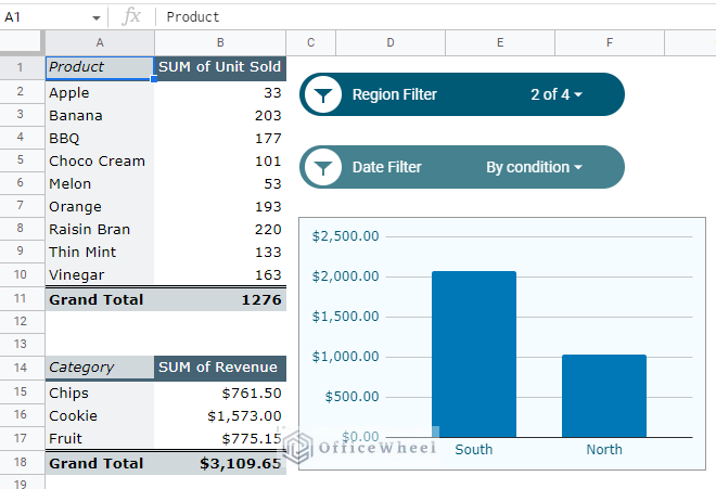
For example, let’s say that we want to see the data of only the North and South regions. So, we check the North and South values in the slicer filter menu.
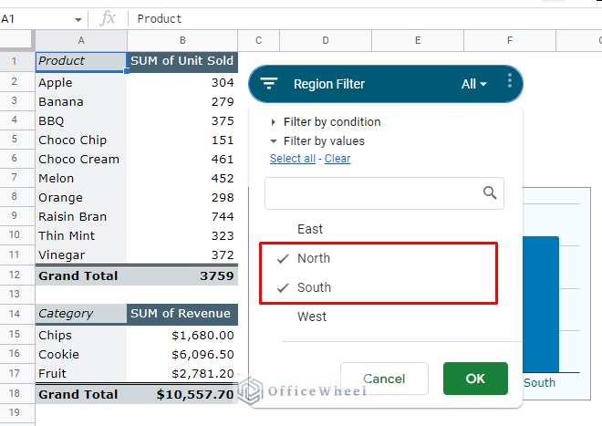
Click OK to see the results.
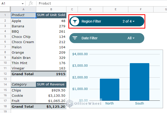
As you can see, not only the pivot tables but also the chart has been updated.
This once again shows the impact of using slicers to filter data in Google Sheets.
2. Filter by Condition (Filter Pivot Table and Chart by Date in Google Sheets)
To customize our filter according to user requirements, we opt for the ‘Filter by condition option’.
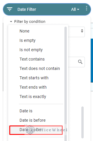
Here, clicking on the drop-down menu will present you with all the default conditions that you can filter by.
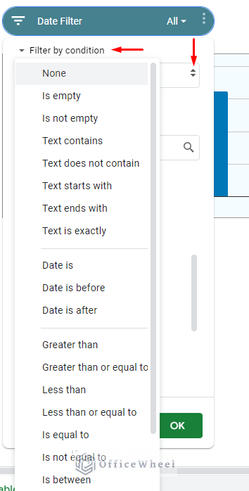
To show off its capabilities, we will try to filter and show only the values that come after the Date of 5/25/2019.
Step 1: Open the drop-down menu and select the ‘Date is after’ option.
Step 2: Open the second drop-down menu and select ‘exact date’. Input the date, which for us is 5/25/2019.
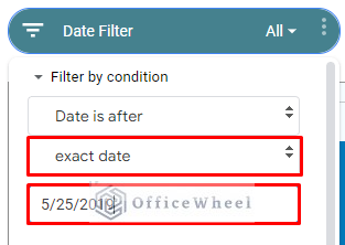
Step 3: Click OK to see the results.
With this, we have also successfully applied multiple filter conditions to a single dashboard.
Final Words
That concludes our simple tutorial on how to use a slicer in Google Sheets. Slicers are a great way to filter data easily into bite-sized pieces that can be utilized by multiple users.
Feel free to leave any queries or advice you might have in the comments section below.