Slicers provide a simple way to filter out data in a spreadsheet. That combined with pivot tables can provide users with a powerful data analysis tool.
So, in this article, we will look at how to add a slicer to a Google Sheets pivot table.
Let’s get started.
What is a Slicer in Google Sheets?
A Slicer (or a Data Slicer) is simply a filter in Google Sheets. That said, it is quite different from the usual filter and has its own set of advantages and uses.
A slicer is a visual filter that can help users manipulate data at a glance with buttons and functions.
When using a filter, the changes are conditionally permanent and cannot be saved for reuse. However, with a slicer, a user can see the data already filtered when they open the worksheet and use the tool anytime to filter data, given that they have access to it.
Another advantage is that slices can be applied to any table or chart, that includes pivot tables.
It is the perfect tool to create a custom dashboard for your team to use at any time.
How to Add a Slicer in a Google Sheets Pivot Table
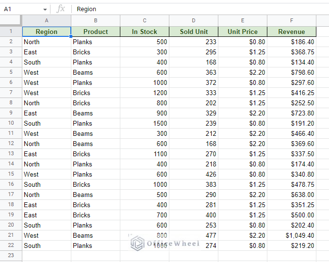
Here we have a sample worksheet that we will use as the source dataset to create the pivot table:
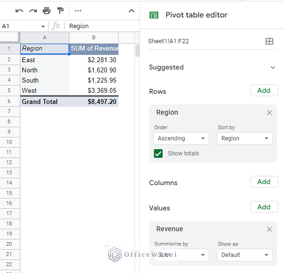
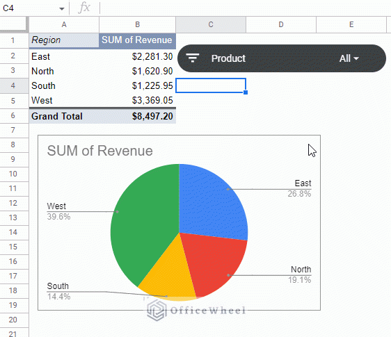
The resultant pivot table shows the Region-wise revenue:
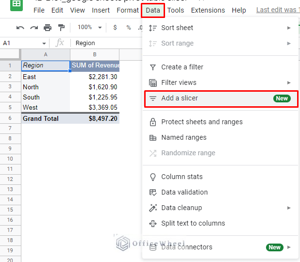
Step 1: To add a slicer to this pivot table, simply navigate to the Data tab and select the ‘Add a slicer’ option.
Data > Add a slicer
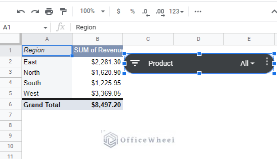
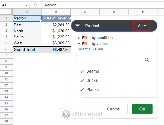
Step 2: The newly generated slicer will then prompt you to select the column option to filter the Google Sheets pivot table by:

We have selected ‘Product’ to be our filter condition.
The slicer automatically recognizes all the headers from the data range used by the pivot table.
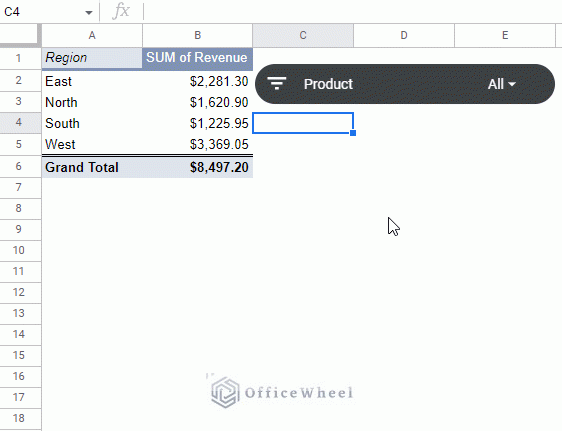
Step 3: The slicer is independent of cell positioning and can be placed anywhere on the worksheet (click and drag).
Place the slicer anywhere suitable.
Step 4: Clicking on ‘All’ will give us the menu. As you can see, the menu is the same as Filters in Google Sheets.
This means that anything you could’ve done with Filters can also be done here.
Setting the Revenue by Region to show the revenues earned by Bricks only:
Example Dashboard Presentation with a Slicer
A more common way to use a slicer is to easily customize the data in a dashboard.
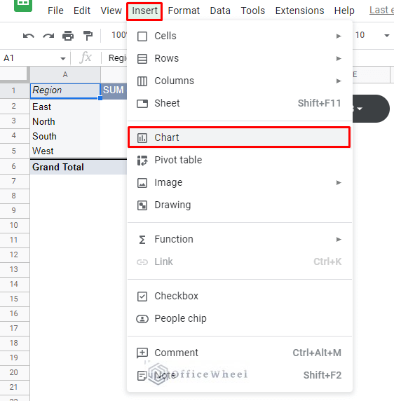
Let’s show that by creating a chart using the pivot table we have now.
Click on any cell of the pivot table and navigate to the Chart option from the Insert menu to insert a chart.
Remove the grand total calculation by updating the range of the chart.
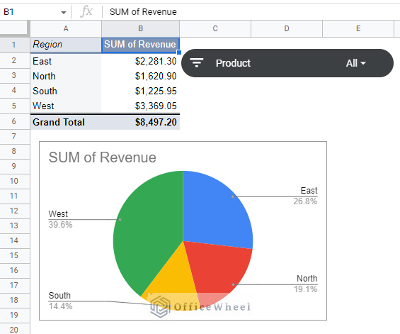
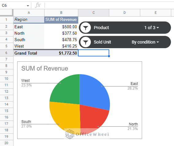
What you see in the above image is a sample dashboard created with a Google Sheets pivot table that includes a slicer filter.
Using the slicer to change the filter conditions will also affect any charts in the pivot table:
You can add Multiple Slicers for a Pivot Table (Multiple Conditions)
It is possible to have more than one slicer for a single Google Sheets pivot table. This means that you can filter your pivot table with multiple conditions.
To add another slicer, just follow the steps we discussed when inserting a slicer in the first place.
Data > Add a slicer
Note: Make sure the data range is correct.
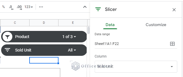
We have chosen the number of Units Sold for the second condition.
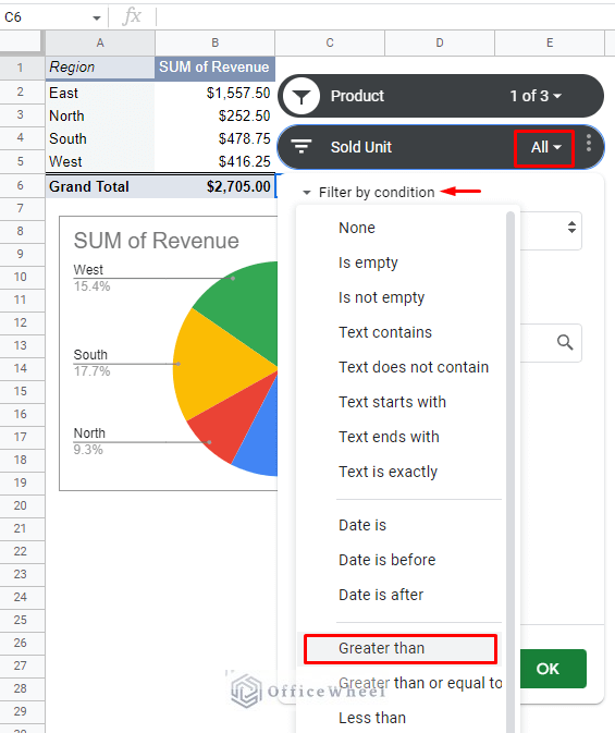
Let’s say we want to filter the revenues of the regions where the number of units sold is greater than 300.
Step 1: Select the ‘All’ drop-down on the second slicer. Click the drop-down ‘Filter by condition’ and select the ‘Greater than’ option.
Step 2: Set the number to 300 and click OK.
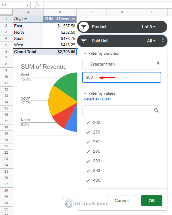
The result:
We have successfully filtered a Google Sheets pivot table with multiple conditions using slicers.
Moreover, you can apply custom conditions to filter in the Google Sheets pivot table slicer.
Final Words
Slicers are the most user-friendly way to set up filters in a Google Sheets pivot table. They follow the same methodology as a normal filter in the application. It even takes the range from the source dataset so applying custom formulas is easy.
On top of that, you can apply multiple slicers to satisfy multiple filter conditions.
Feel free to leave any queries or advice you might have in the comments section below.