With pivot tables being such a powerful data summarization tool, it is no wonder why their use is so widespread. With that popularity, many users may have questions: How do I refresh a pivot table in Google Sheets?
There are multiple ways to approach this, which we will discuss in detail in this article.
But that question comes with a couple more, which we will clarify first.
Do Google Sheets Pivot Tables Automatically Refresh?
Yes. Google Sheets is a browser-based application. This means that every time a change is made to the spreadsheet, the application saves the data automatically.
Whenever this happens, a dependent tool, function, or formula automatically refreshes and updates the data.
And yes, even pivot tables are affected, and their data is automatically refreshed.
Why is the Pivot Table not Updating or Refreshing in Google Sheets?
Even though Google Sheets refreshes every time any data is updated, it is still possible for the pivot table to not update accordingly. There are a few reasons for that:
- The new data entered may be outside the range of the pivot table.
- The pivot table may have filters. Filters sometimes don’t update when a new type of data is entered.
- The source dataset may be using recurring functions or formulas like RAND, TODAY, etc.
These are some of the problems we will solve in this article.
How to Refresh a Pivot Table in Google Sheets
1. Manual Refresh from the Browser
Being a browser-based application, Google Sheets is dependent on a good internet connection.
This also means that any hiccups in the connection may temporarily stop any updates from going through.
So, it is a good idea to occasionally refresh the tab that contains the Google Sheets spreadsheet manually.
You can use the refresh button of the browser (see image below), or use the F5 key of the keyboard.
![]()
Refreshing the browser should also refresh any Google Sheets pivot table as well.
2. Update the Data Range
For this example, we use the following worksheet:
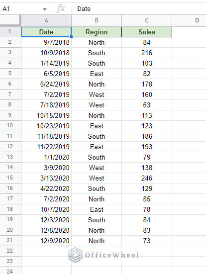
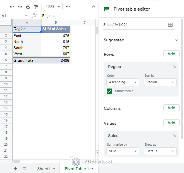
To create the following pivot table:
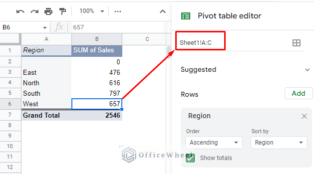
Now, if we enter new data into the table…
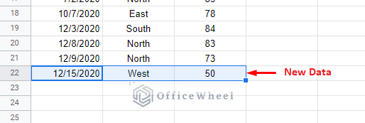
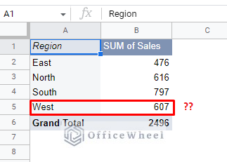
The pivot table does not update (the total sales for the West region should have been 657), why is that?
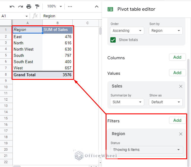
This happens because of the data range of the pivot table. As you can see in the following image, the data range for our pivot table stops at row 21.
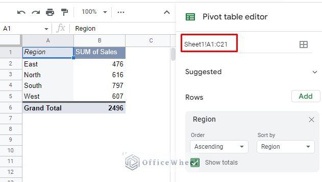
The new data that was entered in row 22, thus, that data was not included in the pivot table.
To refresh and update this data, simply include the new row in the range. The best practice for this is to include the entire columns of data as a range for the pivot table.
Change the range from Sheet1!A1:C21 to Sheet1!A:C.
Now, any new data entered into the source dataset will also be updated in the pivot table every time it is refreshed.
Note: The same can be done for columns.
3. Check Filters of the Pivot Table
We have now entered a few more data into the source dataset:
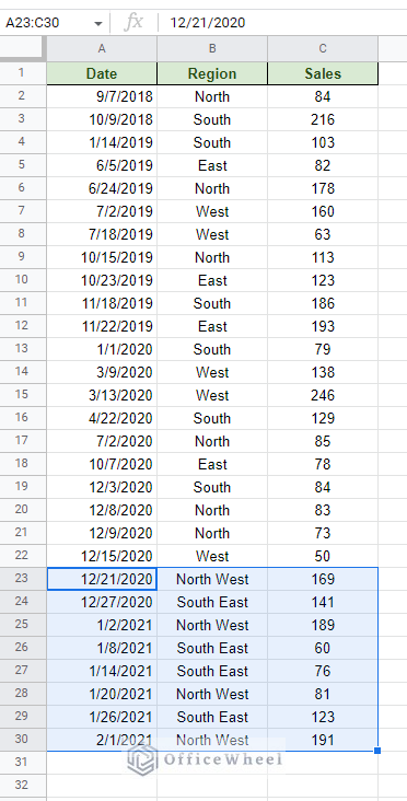
However, these new values don’t show in the pivot table. Even when the data range includes them.
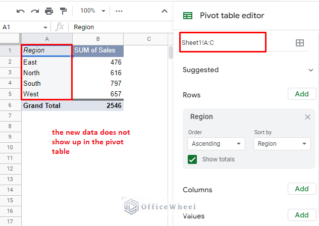
This happens because there is a Filter applied to the Region data of the dataset. We applied this filter initially to remove any blank cells in our pivot table.
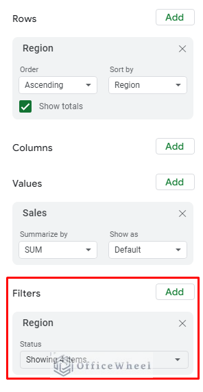
If a Filter is already applied before new data is entered with a new filter condition, the new condition will be unchecked in the filter by default.
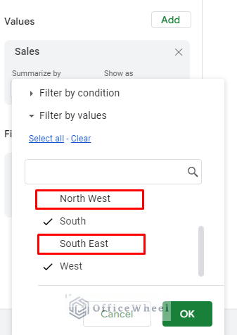
Checking these options in the Filter will make them appear in the pivot table:
Learn More about Filtering Pivot Tables: How to Filter with Custom Formula in a Pivot Table of Google Sheets
Extra: Working with “Running” Functions like RAND, TODAY, etc.
Google Sheets pivot tables don’t work very well with functions that are recurring or need to be refreshed constantly. The functions are RAND, TODAY, NOW, etc. We also call them “running” functions.
Every time the worksheet is refreshed or updated; these values change.
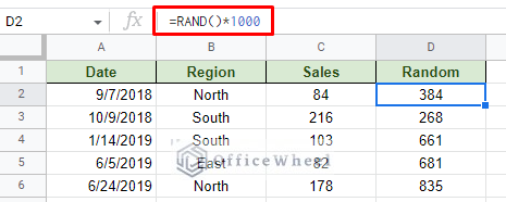
For this example, we have added a column of random numbers using the RAND function and included its sum in the pivot table.
With these functions, every time the worksheet is opened or if any changes are made, the values will update.
We are using F5 to refresh the spreadsheet
However, a lot of strain is put on the spreadsheet due to this constant calculation of data.
Final Words
It is crucial for a pivot table to update itself to always show the latest data. While in most cases, the Google Sheets pivot table will refresh automatically, there are times when it might not happen.
These scenarios are mostly due to the pivot table not including the newly updated cells in its range. Or it can also be due to these data not being included in the Filter. Whatever the case, as long as the user is aware, these issues can be easily remedied.
Please feel free to leave any queries or advice you might have in the comments section below.
Related Articles for Reading
- How to Sort a Pivot Table in Google Sheets (An Easy Guide)
- Pivot Table Formatting in Google Sheets (3 Easy Ways)
- How to Apply and Work with a Calculated Field of a Google Sheets Pivot Table
- How to Group by Month in a Google Sheets Pivot Table (An Easy Guide)
- Using Custom Formula in a Google Sheets Pivot Table (3 Easy Ways)