How to Sort a Pivot Table in Google Sheets (An Easy Guide)

Many ask the question: Can you sort data in a Pivot Table in Google Sheets?

The answer is a resounding yes.

While simple, there is justification to this question, especially if the user is coming from a different spreadsheet application like Excel, where things might have looked and operated differently.

So, the question that remains is how do you sort a Pivot Table in Google Sheets?

That is what we will discuss in this simple guide.

Let’s get started.

How to Sort a Pivot Table in Google Sheets

Basic Sorting with Pivot Table

To show the process of sorting a pivot table, we have the following worksheet:

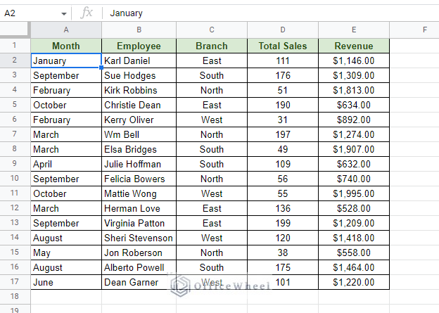
We have simple data that we can use to sort. So, we have decided to create a pivot table and sort total sales by month in Google Sheets.

Step 1: Create a Pivot Table. (Note: You can skip to the next step if you already have a pivot table created in Google Sheets.)

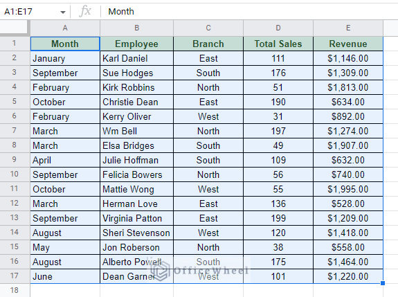
Select the entire dataset, headers must be included:

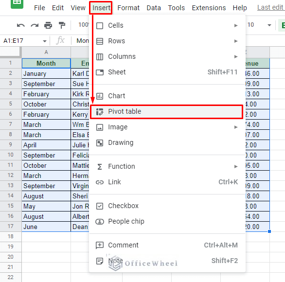
Navigate to the Pivot table option from the Insert tab.

Insert > Pivot table

Select the “New sheet” option to create a new worksheet dedicated to the pivot table. Add the required values for the table (for us it was Row: Month and Value: Total Sales and Revenue). The new Pivot table worksheet will look something like this:

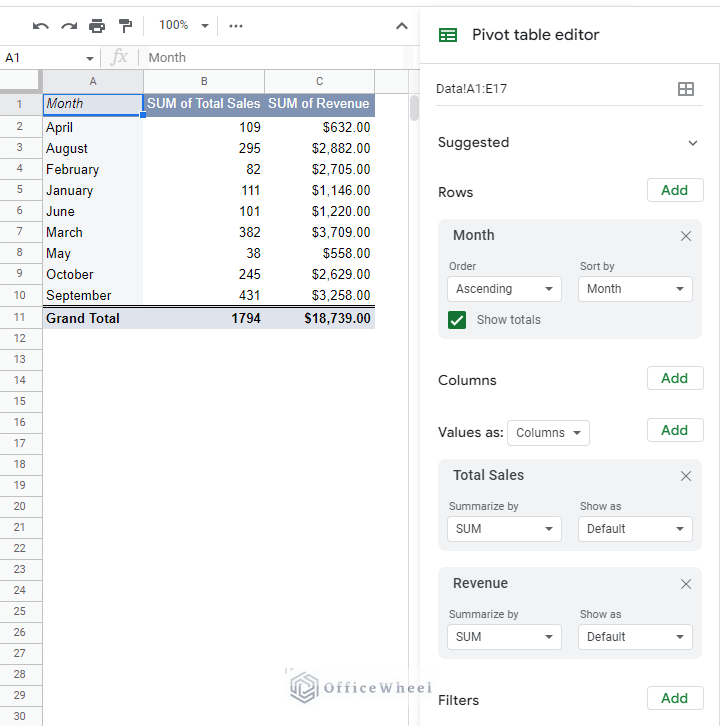
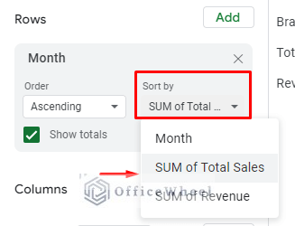
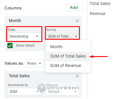
Step 2: Now we get into the first sorting condition. Sorting in Pivot tables is done from the Row section of the editor. And since we are sorting the total sales by months in this Pivot table, our “Sort by” option will be “SUM of Total Sales”.

This is a lot different from Excel where sorting was done via the Sort & Filter option from the ribbon. The pivot table editor of Google Sheets appears to be more intuitive to users.

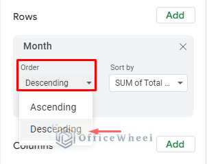
Step 3: The next condition we select is the Order of sorting. Ascending implies that the Total Sales data will be sorted from smallest to largest value, whereas Descending implies that it will be sorted from the largest to the smallest.

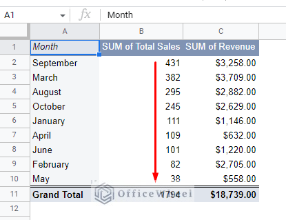
We chose Descending:

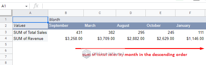
Now, the Pivot Table looks like this when sorted in the descending order of total sales by month in Google Sheets:

Sort by Rows in a Pivot Table

Sorting by rows in a pivot table is similar to sorting by column. Though it depends on the orientation of the data.

In the following pivot table, we have arranged it as such. Like the column orientation seen in the previous section, we have presented the same data in rows this time.

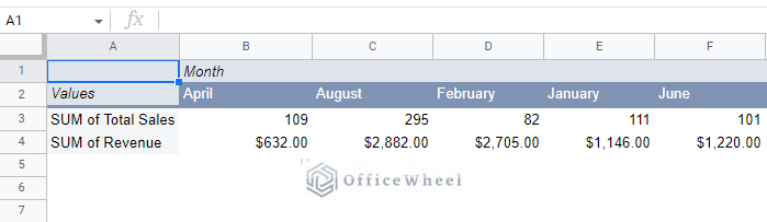
The conditions we have used are also different:

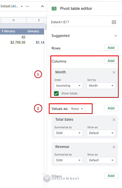
1. Each month is set as a column. This is to get the horizontal orientation.
2. (IMPORTANT!) We must set the value to be presented as Rows, otherwise, there will be an orientation error.

We once again sort by the sum of the Total Sales and in the descending order (largest to smallest).

The result:

Custom Sorting a Pivot Table in Google Sheets

While most sorting tasks of the pivot table can be done right from the editor, some scenarios may require its users to go beyond numerical or alphabetical sorting and move to a more custom priority setting.

Let’s consider the following worksheet example:

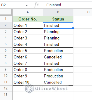
We want to create a pivot table that sorts the data in a custom priority:

Finished > Production > Planning > Canceled

Here are the steps to create a custom sort for a pivot table in Google Sheets:

Step 1: Create a helper column to set the level of priority of the Status values. We create one in column C using the following formula:

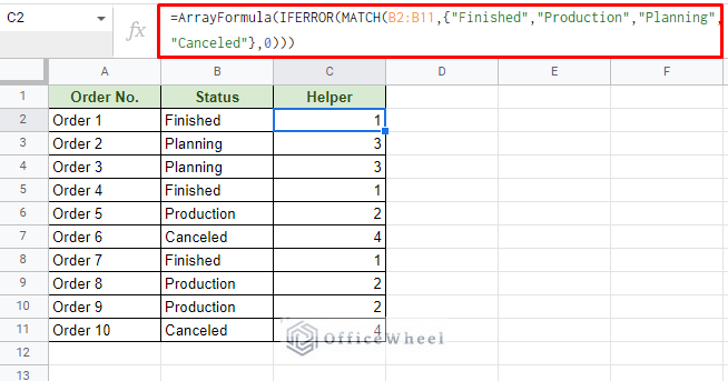
This formula matches the values in the Status column and assigns a numerical value to them in the level of priority. With 1 being the highest and 4 being the lowest here.

Step 2: Create a pivot table with the dataset, either in the same worksheet or a different one. Of course, we must include the helper cell.

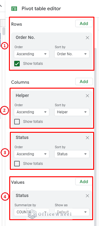
Step 3: Set the following conditions in the pivot table editor.

1. Rows: Add Order No.
2. Columns: Add Helper > Uncheck the “Show totals” box
3. Columns: Add Status > Uncheck the “Show totals” box
4. Values: Add Status > Summarize by COUNTA

You can always see the accompanying image to double-check.

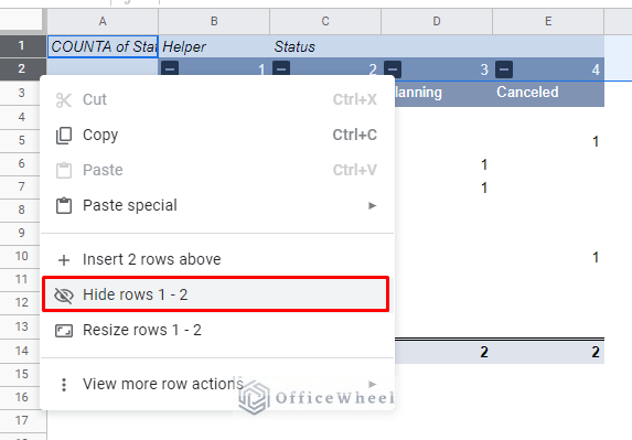
Step 3: We should already have the pivot table sufficiently sorted. But to make it more presentable, we will hide the first two rows of the table.

Select the two rows > Right-click > Hide rows

The resultant Pivot Table:

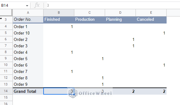
As you can see, the columns are organized in the level of priority. The 1s represent the status of each Order in their respective Statuses. You can also see the total of each order that is in each status in the last row of the table.

Final Words

That concludes our simple guide on how to sort a pivot table in Google Sheets. While most of the sorting tools are already there in the pivot table editor, custom sorting will still require the use of formulas and helper cells.

Feel free to leave any queries or advice you might have in the comments section below.

Related Articles for Reading

• Pivot Table Formatting in Google Sheets (3 Easy Ways)
• How to Apply and Work with a Calculated Field of a Google Sheets Pivot Table
• Using Custom Formula in a Google Sheets Pivot Table (3 Easy Ways)
• Find the Top 10 Values in a Google Sheets Pivot Table (2 Easy Examples)
• Google Sheets Pivot Table: Sort by Value (3 Easy Ways)