
Pivot tables are an amazing tool when it comes to summarizing large amounts of data in Google Sheets. We can further condense our findings by grouping the data according to certain values, like dates.
Thus, in this simple tutorial, we will look at how we can group a pivot table by month in Google Sheets.
Let’s get started.
How to Group by Month in a Google Sheets Pivot Table
Always Validate the Dates First
Dates can be written in many formats in a Google Sheets spreadsheet. However, as spreadsheets change hands and are shared among users, the date format the date is in may become invalid.
While rare, this usually happens due to the different regional settings of the users.
So, when doing calculations revolving around date values, it is crucial to check the validity of the dates in question.
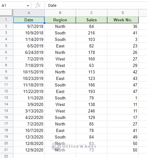
As you can see, the first column contains the date values. To validate these values, all you have to do is go to an empty column and use the DATEVALUE function referencing the cells that contain dates.
=ArrayFormula(IFERROR(DATEVALUE(A2:A),""))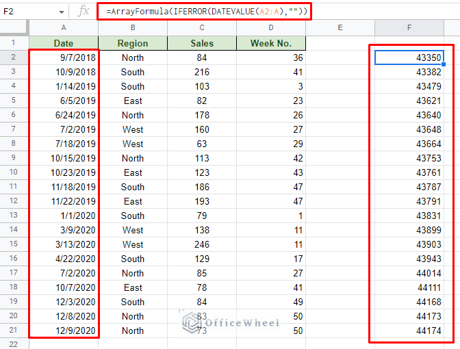
At first glance, the formula may seem a little complicated. But all we did was accommodate the entire Date column (A2:A) in the function and set a handler for any blank cells with IFERROR. You only have to apply this formula in a single cell.
As for the output, you can see we get a numerical value as a result. This indicates that the date is valid.
All that is left is to create a pivot table with this dataset.
Grouping By Month in the Pivot Table
With the pivot table created, we need to populate it with values.
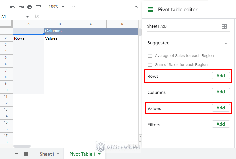
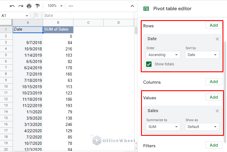
Since we are grouping by dates, more specifically months, we will set the Rows condition from the Date column of the source dataset. We will also use Sales data as Values condition.
Note: You can use Filters to remove the blank cells from Sales.
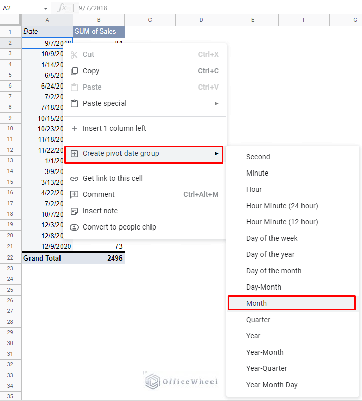
To bring out the group menu, simply right-click over one of the date values and select the option “Create pivot table date group”. From here, you can select the type of grouping you want to do. For the sake of this article, we have chosen “Months”.
To summarize:
Right-click over a date value > Create pivot table date group > Month
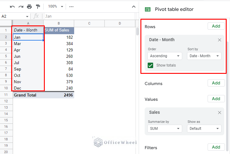
The month grouping that we have just performed for this Google Sheets pivot table shows the sum of sales for specific months in all the years.
So why not also group by years to summarize the data further?
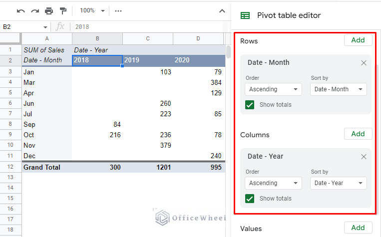
Include Year to the Table
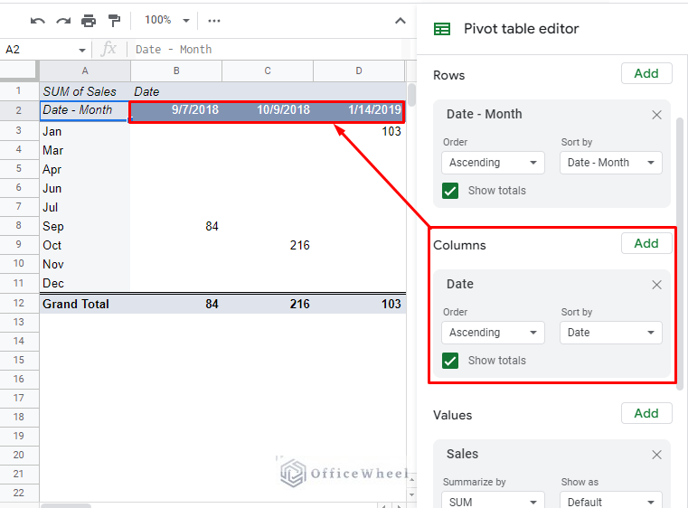
If we want to further summarize by year, we must once again group the dates by years, but not in the same column as months.
Since we already have the months grouped in the primary column, we want to set the other columns as individual years.
Step 1: Set the Columns as Date values.
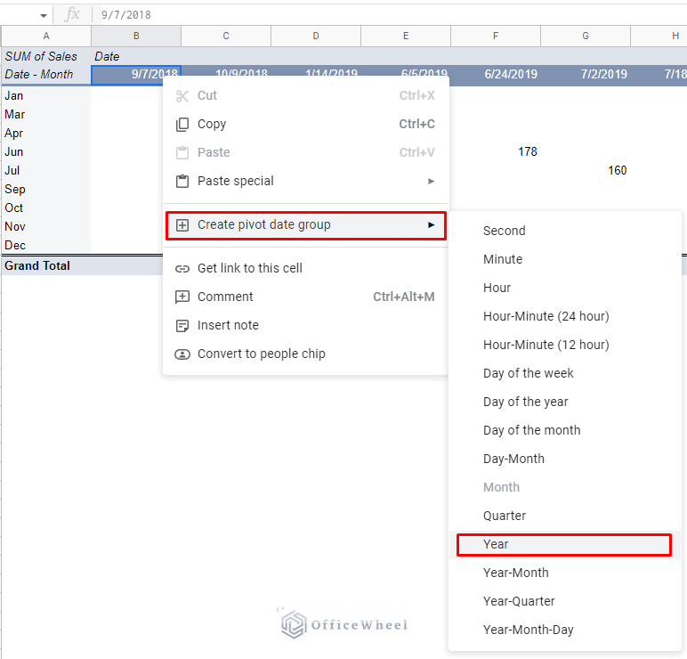
Step 2: Group the columns as years. We will follow a similar procedure as we did with months, but this time, we choose Year.
Right-click over a date value > Create pivot table date group > Year
The result:
Looks much better, doesn’t it?
The data now is much clearer to derive a conclusion from.
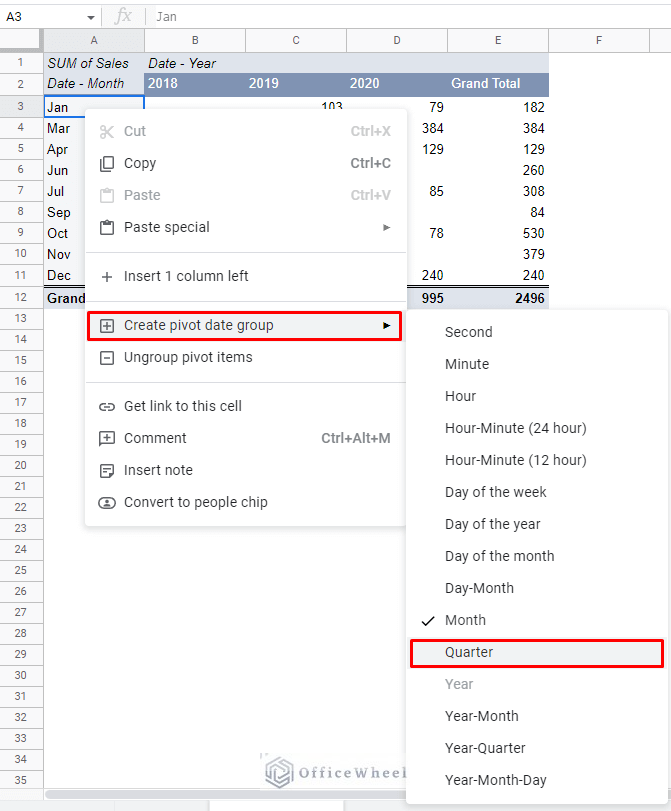
Quarterly Grouping in a Pivot Table in Google Sheets
Another popular form of grouping data in a pivot table is by quarters.
Many organizations, especially those involved in sales, like to analyze their data in quarters of the year. These are:
- Q1: January, February, and March
- Q2: April, May, and June
- Q3: July, August, and September
- Q4: October, November, and December
Thankfully, the option to group a Google Sheets pivot table by quarters is right there in the default group date options. Simply right-click on a date to bring it out:
Right-click over a date value > Create pivot table date group > Quarter
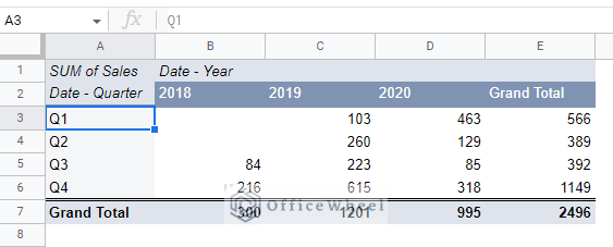
The result:
Final Words
With that, we conclude this simple guide on how to group a pivot table by month in Google Sheets. As long as the date values in the source dataset are valid, we can access the month group option simply by right-clicking over the date data in the pivot table.
Feel free to leave any queries or advice you might have in the comments section below.
Related Articles for Reading
- Google Sheets: Create a Pivot Table with Data from Multiple Sheets
- How to Apply and Work with a Calculated Field of a Google Sheets Pivot Table
- Using Custom Formula in a Google Sheets Pivot Table (3 Easy Ways)
- Pivot Table Formatting in Google Sheets (3 Easy Ways)
- How to Sort a Pivot Table in Google Sheets (An Easy Guide)