How to Filter with Custom Formula in a Pivot Table of Google Sheets

Pivot tables are perhaps one of the best data presentation tools available in any spreadsheet application. Which brings us to today’s question: Can you filter a pivot table in Google Sheets with a custom formula?

The answer is, of course, yes. Using custom formulas will open a new horizon to the filtering capabilities of the application, which includes the pivot table.

Filter with Custom Formula in a Pivot Table of Google Sheets

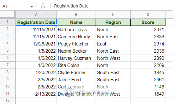
For our example, we have created the following dataset…

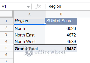
And its corresponding pivot table showing the Scores by Region:

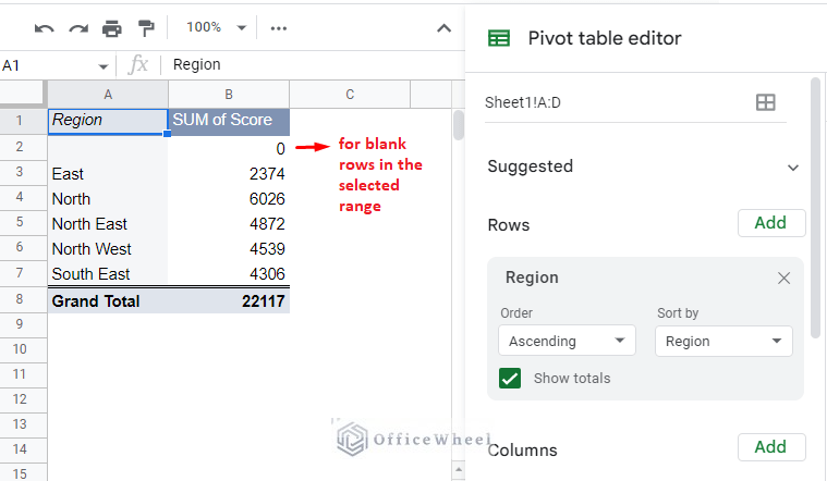
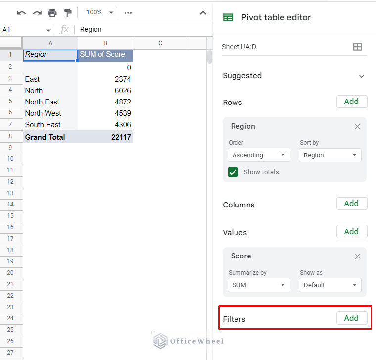
By default, Google Sheets pivot table editor already provides us with a Filter option to filter data. We can find this option near the bottom of the editor.

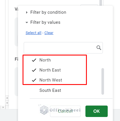
Let’s say we want to filter all the scores by Regions that contain ‘North’.

Add Filter > Region > Status > Select all options containing ‘North’

The result:

In most cases, this type of filter is enough. But when it comes to filtering our more specific data with conditions, the default option has some limitations.

Limitations of the Regular Pivot Table Filter

Let’s consider the scenario where we want to find all the regional scores by Registration Date in the pivot table of Google Sheets. The filter condition will be all dates after 2/1/2022.

Now, if we go to do a default Filter by Date, we will get something like this:

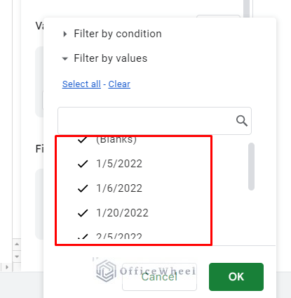
All the individual date entries are listed. This means that every time we add a new date a new option will be registered.

This makes the regular filter of the pivot table quite inefficient when handling conditional data like greater than or less than.

But thankfully, we can use custom formulas to filter in a pivot table of Google Sheets.

Simple Custom Formula for Filtering in a Pivot Table (Filtering Dates)

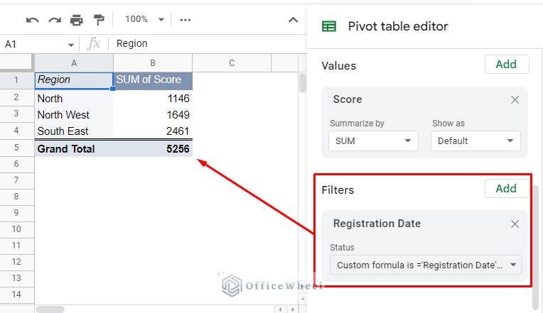
Let’s return to the filter condition of presenting scores by region after the date 2/1/2022 in a pivot table. This time, we will use a custom formula to apply the condition.

Step 1: Add Registration Date in the Filter section of the Pivot table editor.

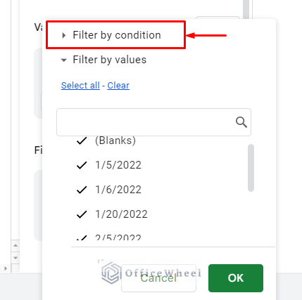
Step 2: Click the drop-down under the Status field. This will bring out all the available condition options. Select the ‘Filter by condition’ option.

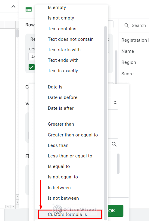
Step 3: Scroll down to the bottom to find and select the “Custom formula is” option.

Step 4: Enter the following custom formula:

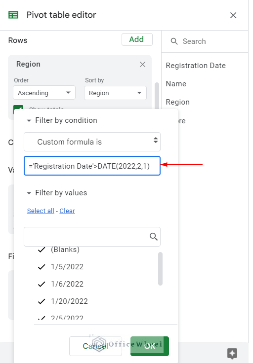
Formula Breakdown:

• ‘Registration Date’: The name of the header from which we get the date values. This header reference must be inside single quotes (‘’). Note: All the header names of the source dataset are listed on the right side of the Pivot table editor.
• >: The greater than condition. We can also use “>=” to include the starting date.
• DATE(2022,2,1): The date reference for the starting date. We have used the DATE function to avoid any formatting error of the date input.

Step 5: Click OK to apply the custom formula.

Advantages of using a Custom Formula as a Filter for a Pivot Table

1. A user can apply any conditions.
2. Any number of conditions can be applied
3. The user can use the formulas with cell references. Has all the advantages of using cell references like locking row or column references.
4. The formulas are fully customizable thanks to the ability to use regular expressions.

Using Regular Expression Custom Formula to Filter in a Pivot Table

Regular expressions are perhaps the single best way to customize any conditions for formulas in Google Sheets. Let’s show what we mean through an example.

Let’s say we want to filter the pivot table to show data from all East regions. This will include North East or South East regions. Basically, any region data that contains the text ‘East’.

But before we get into the pivot table, let’s show you what happens when we search for ‘East’ using a formula without regular expressions. The formula is:

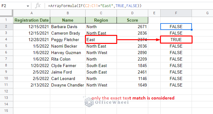
All cell values that do not contain the exact text match are shown as FALSE. Unless we include the other values that contain ‘East’, the general formula will not work for our condition.

Now let’s do the same with a regular expression function: REGEXMATCH. This works similarly to the previous IF function to search the range and match the given value. The formula:

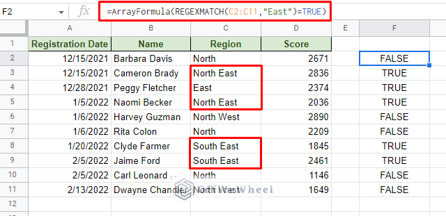
The REGEXMATCH function acts similarly to IF to find the correct match. But this time, the function also works for partial matches (it is still case-sensitive though). This is one of the biggest advantages of using regular expressions.

Now, let’s apply a formula similar to this for the pivot table filter custom formula in Google Sheets:

Step 1: In the Pivot table editor, select Region as the filter. Like before, select the “Custom formula is” option.

Add Filter: Region > Status > Filter by condition > Custom formula is

Step 2: Input the following custom formula:

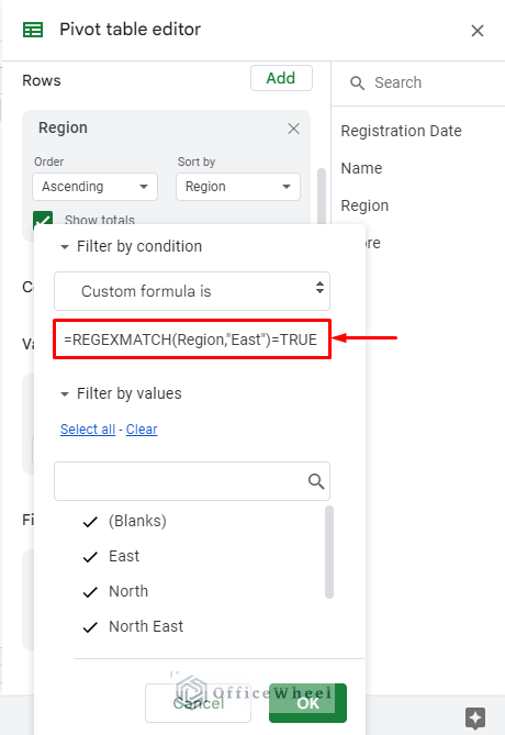
Note that instead of a cell range we have put the column header name (Region) for the text/range argument for the REGEXMATCH function. This is what you have to do in pivot tables. It is simple and easy to apply.

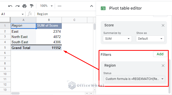
Step 3: Click OK to apply the filter.

Filter with Multiple Conditions in Pivot Table

Another advantage of using regular expressions is that you can add more of the same type of conditions in the same formula.

For example, let’s say that we want to include the ‘West’ as a condition as well. With a small update, the formula will look like this:

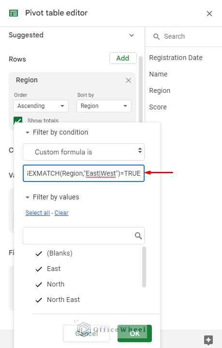
This is the OR symbol (|) for regular expressions. This sets the condition for including either ‘East’ or ‘West’ in the filter.

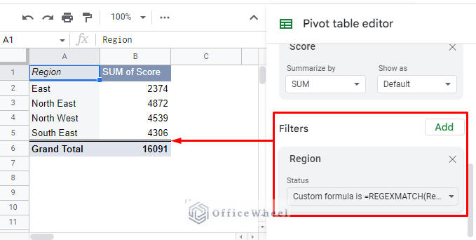
The result:

Final Words

Using a custom formula to filter data in a pivot table of Google Sheets is not only easy but also quite useful. Thanks to formulas being so customizable in Google Sheets, there are virtually no limits to the filtering conditions that a user can apply.

Feel free to leave any queries or advice you might have in the comments section below.

Related Article for Reading

• How to Sort a Pivot Table in Google Sheets (An Easy Guide)
• Pivot Table Formatting in Google Sheets (3 Easy Ways)