Adding some cells from a row, column or array is one of the most common things one can do in Google Sheets. The SUM function in Google Sheets can be utilized in such cases. The SUM function can add numbers, numbers stored as texts, or unique numbers stored for text values. Here, in this article, I will demonstrate a few examples of how to use the SUM function in Google Sheets.
A Sample of Practice Spreadsheet
What Is SUM Function in Google Sheets?
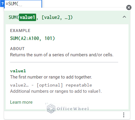
The SUM function is used to return the sum of a series of numbers and/or cells.
Syntax
The SUM function’s syntax is as follows:
=SUM (value1, [value2, ...])Arguments
| Argument | Requirement | Function |
|---|---|---|
value1 |
Required | The first number or range to add together |
[value2] |
Optional | Additional numbers or ranges to be added to value1 |
Output
The formula SUM (3,5,8) will have an output of 16.
6 Examples to Use SUM Function in Google Sheets
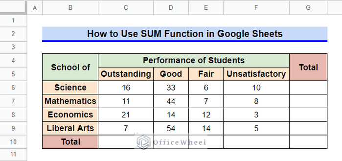
First, let’s know about our dataset. We have considered the performance of students from four different schools. Here, we can apply the SUM function to determine the total number of students from various categories. Now, let’s go through the examples.
1. Add Values Directly
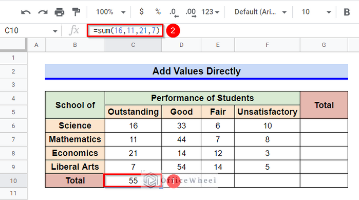
Here, we will calculate the total number of students who have outstanding performance.
Steps:
- For that, go to Cell C10 (where you want to calculate the total) and type the following formula, and press Enter key-
=SUM (16,11,21,7)Read More: How to Add Up A Column in Google Sheets
2. Sum Up Cells of a Row
Entering every value like in the previous method isn’t very efficient in large datasets. Also, changing any value from the dataset will not change the value of the output. We can insert the values as a range instead to create a more flexible and dynamic dataset.
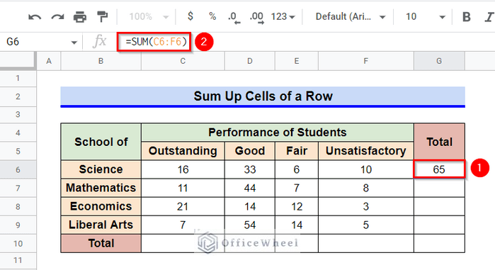
Here, I’ll be calculating the total number of students in the School of Science.
Steps:
- For that, go to Cell G6 and type in the following formula and then press Enter key-
=SUM (C6:F6)Here, the array C6:F6 indicates the value of every cell from Cell C6 to Cell F6.
Read More: Google Sheets: Sum If there are Multiple Conditions (3 Ways)
3. Add Cells of a Column
Here, we will use the SUM formula to calculate the total number of students in consideration.
Steps:
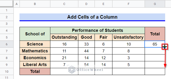
- Follow the previous method to calculate the total number of students in the School of Science. Then use the Fill Handle icon to copy the formula into other cells of the column.
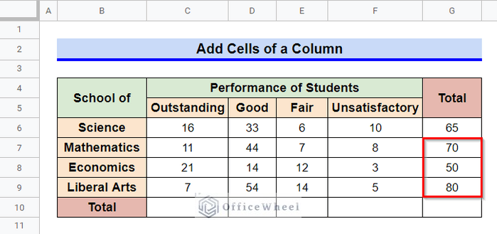
- This will calculate the total number of students in other schools.
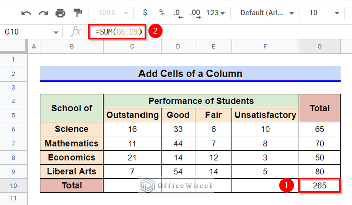
- Now, in Cell G10, type in the following formula and press Enter. This will calculate the total number of students in consideration-
=SUM(G6:G9)Read More: Google Sheets: Sum an Entire Column (4 Easy Ways)
Similar Readings
- How to Sum Cells from Different Sheets in Google Sheets (3 Easy Ways)
- Google Sheets: If Cell Color is Red Then Take Action
- How to Link Cells Between Tabs in Google Sheets (2 Examples)
- Copy and Paste Formulas in Google Sheets (4 Easy Ways)
4. Add Specific Cells
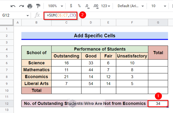
We can use the SUM function to exclude a few cells while adding the values from a range. For example, let’s calculate the number of students who have outstanding performance but are not from the School of Economics.
Steps:
- To calculate this, go to Cell G12 and type in the following formula and then press Enter Key-
=SUM(C6:C7,C9)Read More: Find the Sum of Cells with Specific Text in Google Sheets
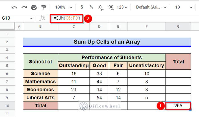
5. Sum Up Cells of an Array
We can include both rows and columns in our range for the SUM formula.
Steps:
- Instead of method 3, we can type the following formula in Cell G10 and press Enter key to calculate the total number of students in consideration-
=SUM(C6:F9)6. Sum Unique Numbers Stored for Text Values
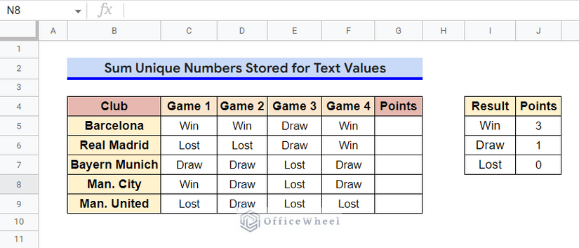
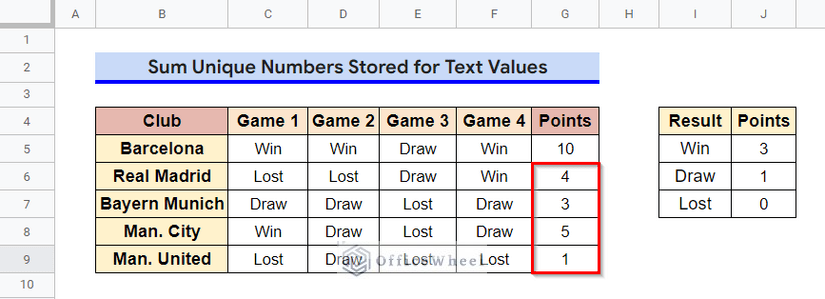
We can use the SUM function combined with the VLOOKUP function and the ARRAYFORMULA function to add unique numbers stored for text values. For that, we have taken a new dataset where the result for 4 different games is shown for 5 different clubs. The points assigned for each type of result are also indicated in a different table. We need to calculate the total points for each club.
Steps:
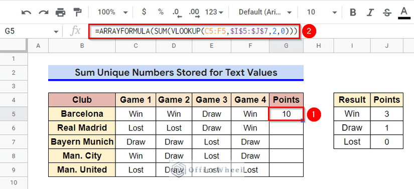
- Select Cell G5 and type in the following formula and then press Enter key.
=ARRAYFORMULA(SUM(VLOOKUP(C5:F5,$I$5:$J$7,2,0)))Formula Breakdown:
- VLOOKUP(C5:F5,$I$5:$J$7,2,0)
The VLOOKUP function searches down the first column of the range I5:J7 for search key C5:F5 and return specified cells from 2nd column of the range.
- SUM(VLOOKUP(C5:F5,$I$5:$J$7,2,0))
Next, the SUM function returns the sum of the numbers returned by the VLOOKUP function.
- ARRAYFORMULA(SUM(VLOOKUP(C5:F5,$I$5:$J$7,2,0)))
After that, the ARRAYFORMULA function helps the non-array function VLOOKUP to return an array to the SUM function.
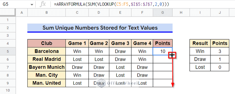
- Now, use the Fill Handle to copy the formula in other cells of the column.
- Thus, we can sum unique numbers stored for text values.
Read More: How to Use ARRAYFORMULA with VLOOKUP in Google Sheets
How to Automatically Add Numbers in Google Sheets
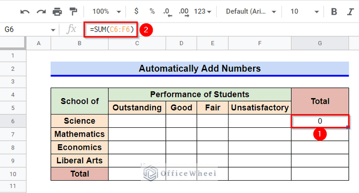
One can add numbers automatically with every entry in the datasheet if he/she types the formula before entering the values.
Steps:
- Select Cell G5 and type in the following formula and press Enter key. Since there is no entry yet in the array C6:F6 the output is 0.
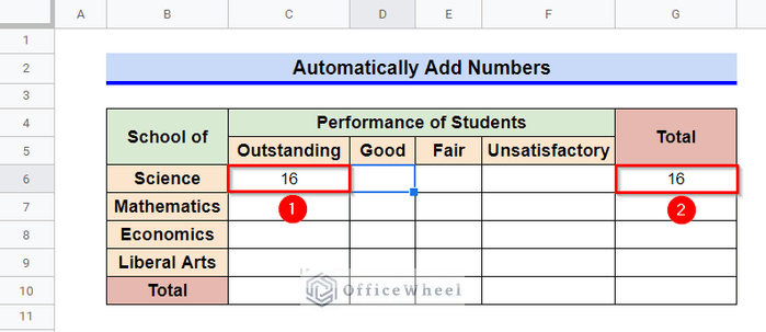
=SUM(C6:F6)- Now, select Cell C6 and start entering data for the array. As soon as you enter the data in Cell C6 and press Enter or Tab key, the value in Cell G10 will change.
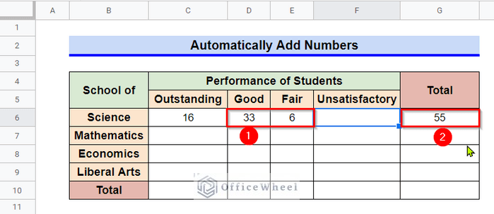
- Each time you enter/change a value in that array, the value in Cell G6 will also change.
Read More: How to Automatically Add Numbers in Google Sheets
What to Do When SUM Function Is Not Working in Google Sheets
Sometimes some formulas in Google Sheets might not show the required result although every argument of the formula has been inserted correctly. There can be various reasons behind this problem. But here we discuss one of the most common instances where the SUM function doesn’t provide the required output and how we can solve this problem.
Steps:
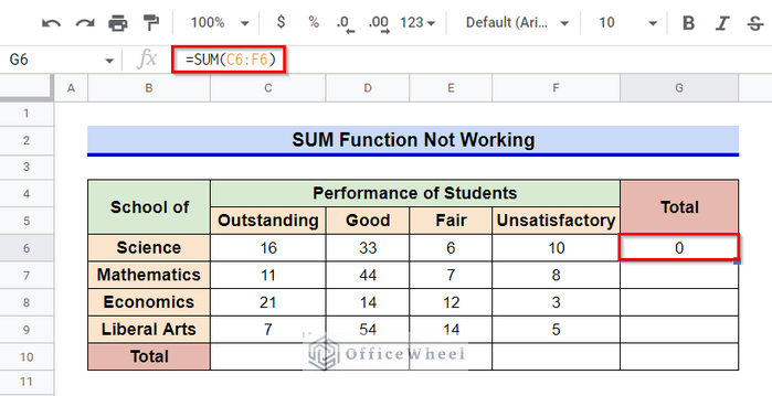
- Here, in this datasheet, we have inserted the arguments correctly in the SUM function; but instead of the accurate output of 65, the SUM function has provided us with an output of 0.
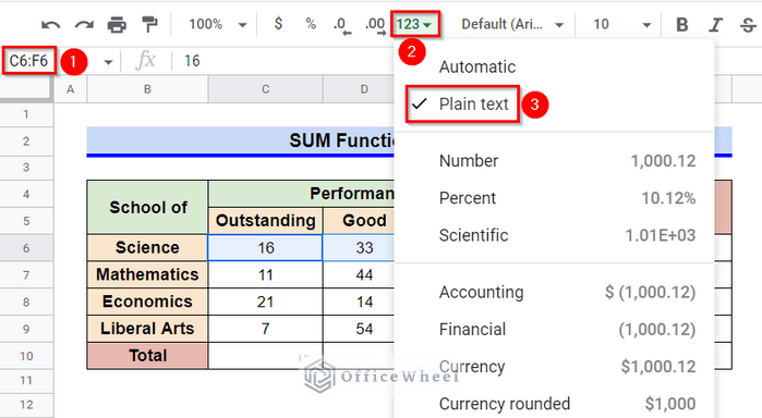
- But if you select the array of the argument and go to the More Formats option from the Clipboard, you will see that instead of Number or Automatic, the data format is Plain Text. This is the reason behind an output of 0.
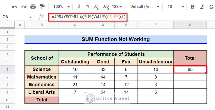
- Now, we can change the format to Automatic or Numbers. But instead of changing the dataset, we can combine the SUM function with the ARRAYFORMULA function and the VALUE function to calculate the sum. For that, select Cell G5 and type in the following formula, and then press Enter key.
=ARRAYFORMULA(SUM(VALUE(C6:F6)))Formula Breakdown:
- VALUE(C6:F6)
The VALUE function converts the string entries into numbers.
- SUM(VALUE(C6:F6))
Then the SUM function adds the numbers returned by the VALUE function.
- ARRAYFORMULA(SUM(VALUE(C6:F6)))
Finally, the ARRAYFORMULA function helps the non-array function VALUE to return an array to the SUM function.
Read More: How to Sum Using ARRAYFORMULA in Google Sheets
Things to Be Considered
- Use Comma (,) between arguments of the SUM function.
- Use the ARRAYFORMULA function in cases where a non-array function has to return an array.
Conclusion
This concludes our article to learn about how to use the SUM function in Google Sheets. I hope the provided examples will be sufficient for your requirements. Feel free to leave any comments or advice in the comment box.
Related Articles
- How to Use IF and OR Formula in Google Sheets (2 Examples)
- Use ARRAYFORMULA in Google Sheets (6 Examples)
- How to Use ARRAYFORMULA with IF Function in Google Sheets
- Google Sheets: How to Autofill Based on Another Field (4 Easy Ways)
- How to Auto Sum in Google Sheets
- Sum Multiple Rows in Google Sheets (3 Ways)
- How to Sum Colored Cells in Google Sheets (2 Ways)

