In this simple tutorial, we will look at a few ways to find the sum of cells with specific text in Google Sheets.
While it sounds simple, there are multiple other conditions to consider, like:
- Do you want to match the text of the whole cell?
- Do you want a partial match of text from the cell?
- Is there more than one text condition to look for?
Each of these scenarios warrants customization to the base formula. But luckily the base function that we will use is the same: SUMIF.
The Core Function: SUMIF
The SUMIF function is the perfect function for this scenario for the exact two reasons we need it for: Summing with a Condition.
The SUMIF function syntax:
SUMIF(range, criterion, [sum_range])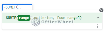
Let’s show how it works with a simple example.
Note: You can skip ahead to the methods if you already understand the fundamentals of the SUMIF function.
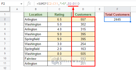
Here, we have a simple SUMIF application where we sum the number of Customers for the Location Rating greater than 5:
=SUMIF(C2:C11,">5",D2:D11)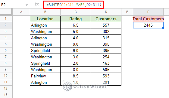
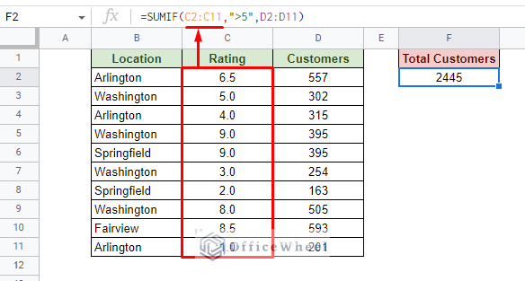
First, C2:C11 is the range where our criterion lies:
Next, “>5” is the criterion that we will look for in the range.
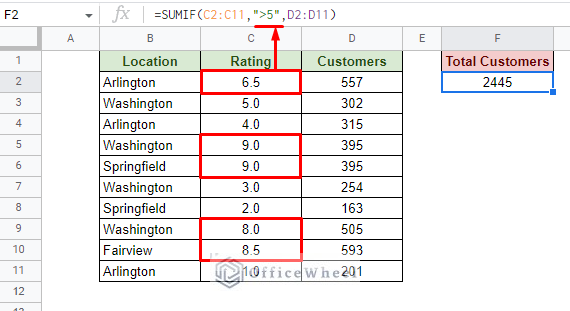
Finally, D2:D11 is the sum_range whose values are added when their respective cell matches the criterion.
With the fundamentals out of the way, let’s get into the different scenarios.
4 Ways to Find the Sum of Cells with Specific Text in Google Sheets
1. Sum of Cells with Exact Text Match
For this scenario, we have the following dataset of Locations and their respective Customers:
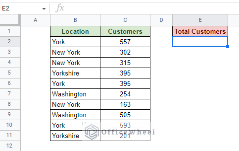
We want to find the total number of customers for the location “York”.
The formula is:
=SUMIF(B2:B11,"York",C2:C11)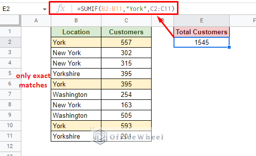
As you can see, while there are a lot of “York”s in the list, only the cells that have the exact match of the given word are counted.
Depending on the situation, this can be considered to be both an advantage and a disadvantage.
2. Sum of Cells with Specific Partial Text Match in Google Sheets
Looking for partial text matches is much more common in a spreadsheet. The core of this search approach is to use the asterisk operator (*) with the criterion text depending on its position in the cell.
Here are 3 such scenarios:
I. Cell Starts with Specific Text
For this example, we will find the sum of Customers for cells that start with the text “York” in Google Sheets.
As long as the text in the cell begins with “York” whatever appears after is fine. This means that the asterisk operator will go after the text: “York*”.
The formula:
=SUMIF(B2:B11,"York*",C2:C11)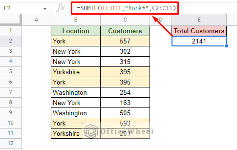
Here, both York and Yorkshire were included since they both start with the string “York”.
II. Cell Ends with Specific Text
The only difference here from the previous method will be the position of the asterisk operator (*).
Since we are looking for cells that end with “York” the asterisk will be placed at the beginning of the string to represent the acceptance of all characters before: “*York”.
The formula is:
=SUMIF(B2:B11,"*York",C2:C11)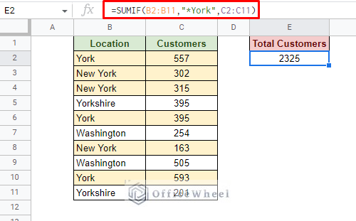
Here, both York and New York were included since they both end with the string “York”.
III. Cell Contains Specific Text in General
If you are looking for a text anywhere in the cell, this is the approach for you.
All you have to do is place the asterisk operator (*) on both ends of the desired text in the criterion field of SUMIF.
For example, if we want to find the sum of cells with the specific text “York” in Google Sheets, the criterion condition will be: “*York*”.
The formula is:
=SUMIF(B2:B11,"*York*",C2:C11)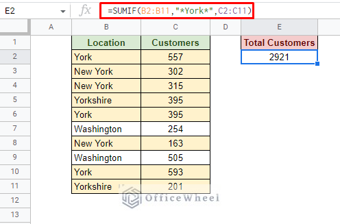
Placing the asterisk on either side allows the SUMIF function to consider any character before or after the text. Since the location York is the exact match in the cell, it is included in all cases.
Note: all of the text criteria are case insensitive.
Reference Another Cell for the Specific Text
Continuously typing in different criteria to sum can prove to be quite tedious in the long run.
So that’s why instead of always updating the formula, it is best to set the formula to reference another cell for the criterion.
For example, here we refer to cell G2 for the keyword “York” as the criterion for SUMIF:
=SUMIF(B2:B11,G2,C2:C11)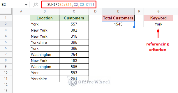
What we’ve just shown is the exact match of the criterion.
For a specific text criterion, in other words adding the asterisk operator (*), will have a different process in this scenario.
We cannot simply include the asterisk on either side of the cell reference:
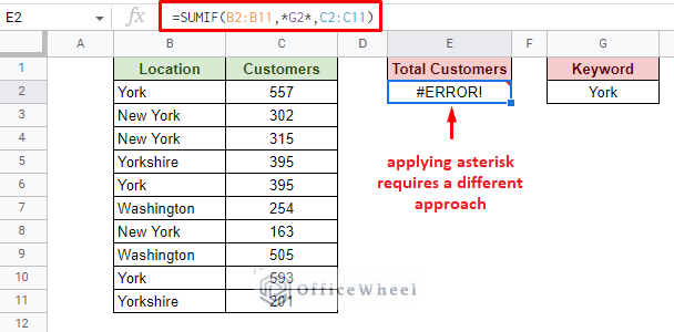
This is because the asterisk (*) is a text value whereas a cell reference is not.
Instead, we must concatenate the two so that they both operate as the same value. For this, we will use the ampersand operator (&).
Thus the criterion will look something like this:
"*"&cell_reference&"*"We are simply including the asterisk symbol on both sides of the referenced value.
Thus, the formula becomes:
=SUMIF(B2:B11,"*"&G2&"*",C2:C11)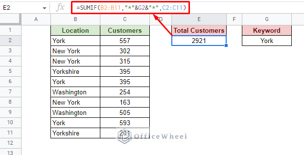
Other applications of the asterisk will also work.
3. Further Use of Wildcards to Sum Cells with Specific Text in Google Sheets
The asterisk symbol (*) that we’ve used in the previous method is a type of wildcard character in Google Sheets.
Wildcards are special characters that help convey certain text conditions alongside text criteria in many functions.
Along with the asterisk, two other notable wildcards are:
- Question Mark (?)
- Tilde (~)
How to Use the Question (?) Wildcard with SUMIF
The question (?) wildcard represents any single character of a text string in Google Sheets. This also includes whitespaces.
For this example, we have the following worksheet:
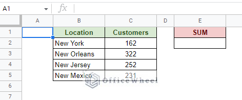
While all of the Location data starts with “New”, they end in different texts.
So, if we sum with criteria “New” followed by seven “?”, we get:
=SUMIF(B2:B5,"New???????",C2:C5)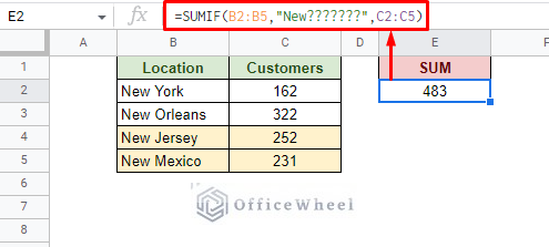
Here, New Jersey and New Mexico were selected since both Jersey and Mexico are 7 characters including the preceding whitespace.
The other two locations don’t meet the criterion and thus are not included in the sum.
We can also combine multiple wildcards at once to set up complex lookup conditions.
For example, setting the criterion to “N*o?*” will make the function look for text that starts with “N” and an “o” which is not the last character of the cell:
=SUMIF(B2:B5,"N*o?*",C2:C5)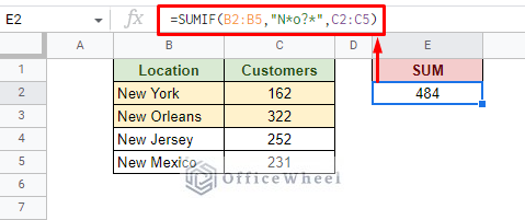
While New Mexico has an “o” as well, it is not counted since the “o” is the last character of the text.
How to Use the Tilde (~) Wildcard with SUMIF
Some wildcard characters may appear in the text of the range of cells that the function is looking up, of which the question mark (?) is common.
In some cases, the “?” may be the character we are looking for as a criterion. But on its own, this character conveys a different meaning.
=SUMIF(B2:B5,"New ?",C2:C5)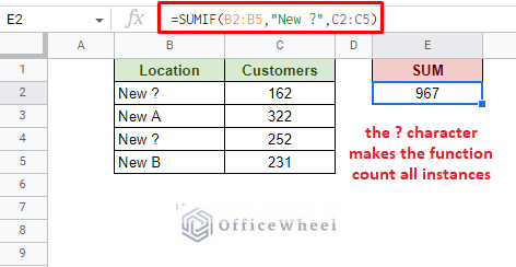
In comes the tilde (~) wildcard.
This allows functions to look up characters that would otherwise be considered a wildcard criterion.
Formula to sum all cells that contains “?” as a text in Google Sheets:
=SUMIF(B2:B5,"New ~?",C2:C5)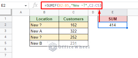
4. Sum Cells with Multiple Text Criteria in Google Sheets
It is not uncommon to have more than one criterion to sum values within Google Sheets.
While SUMIF can take only one criterion, we have the SUMIFS function that can handle multiple:
SUMIFS(sum_range, criteria_range1, criterion1, [criteria_range2, criterion2, ...])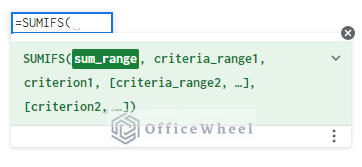
For this example, consider the following worksheet:
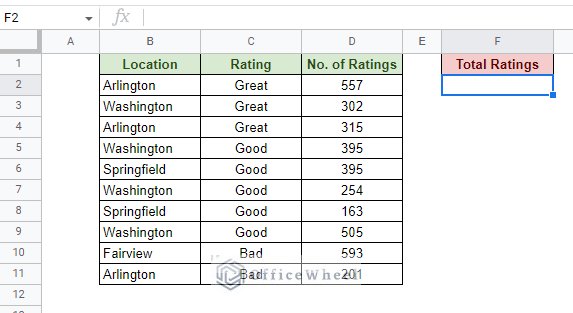
Here, we want to find the total number of ratings for “Good” ratings coming from “Washington”.
Both of these conditions come from different columns: Location and Rating. And the sum range will be the No. of Ratings column.
Making the formula:
=SUMIFS(D2:D11,C2:C11,"Good",B2:B11,"Washington")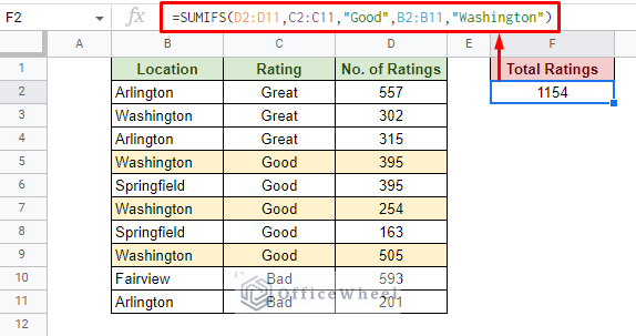
Where:
- D2:D11 is the sum range from the No. of Rating column.
- C2:C11,”Good”: Text criterion for the Rating column.
- B2:B11,”Washington”: Text criterion for the Location column.
Note: For all three ranges, we can remove the lower row limit (e.g., D2:D11 to D2:D) to make the function more dynamic and accept new entries.
Final Words
That concludes all the scenarios and methods we can employ to find the sum of cells with specific text in Google Sheets.
The core of all the methods lies in the use of the SUMIF function and its multi-criteria variant, the SUMIFS function.
Feel free to leave any queries or advice you may have for us in the comments section below.