Google Sheets: If Cell Color is Red Then Take Action

In this article, we will look at a few ways to work with the condition “if cell color is red the take action” in Google Sheets.

With conditional formatting being so widely used in Google Sheets, it is no wonder that many users would want to build up and try to extract more information from these colored cells.

And with the color red in its various forms is widely used to represent certain data, making it quite common to come across in a spreadsheet.

Combining these two scenarios and working with them is what we will focus on in this article.

Note: The methods we will discuss here will work with ALL COLORS.

2 Ways to take Action if Cell Color is Red in Google Sheets

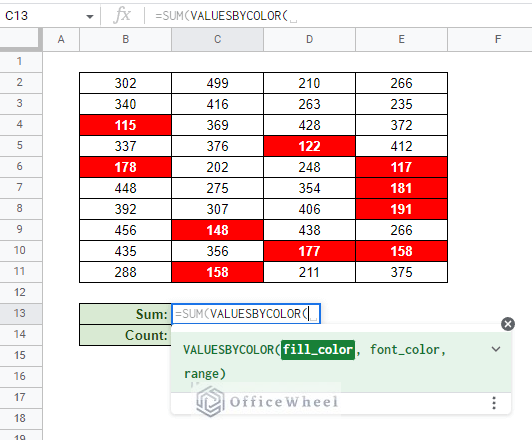
To show the methods, we will use the following worksheet:

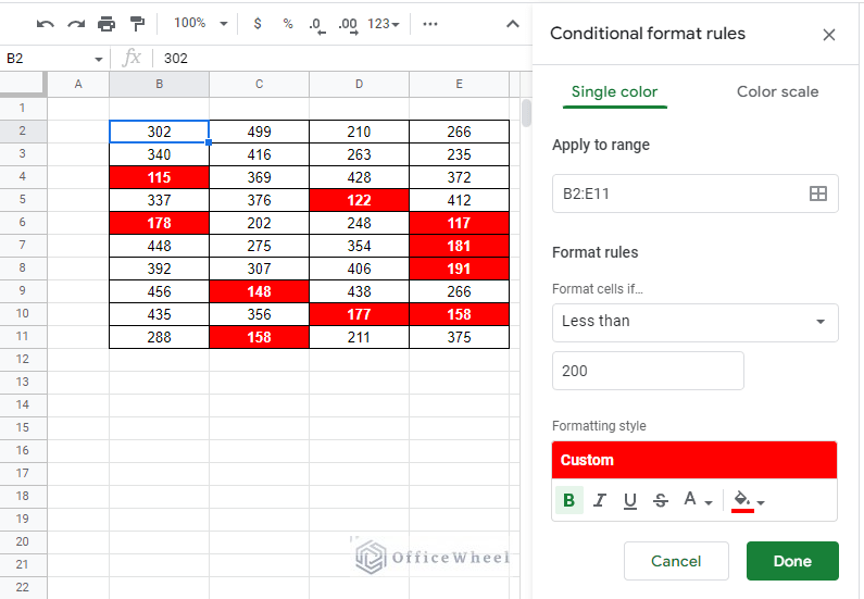
All the numbers that are below 200 are highlighted in red with the help of traditional conditional formatting.

Using this information, we will be performing two actions if the cell color is red in Google Sheets:

1. Sum the cells that are red colored.
2. Count the number of cells that are red-colored.

Let’s get started.

1. Employ Add-Ons to Work with Cell Color in Google Sheets

The add-on in question is called Function by Color. It is a small feature-packed part of the Power Tools add-on of Google Sheets.

Having either of them will work for this topic. Not to mention, they are both free to use at least for the features we need.

Simply follow these steps to get the add-on installed on Google Sheets. If you already have it, skip to the next section.

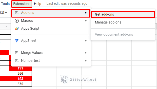
Step 1: Navigate to the Get add-ons option from the Extensions tab.

Extensions > Add-ons > Get add-ons

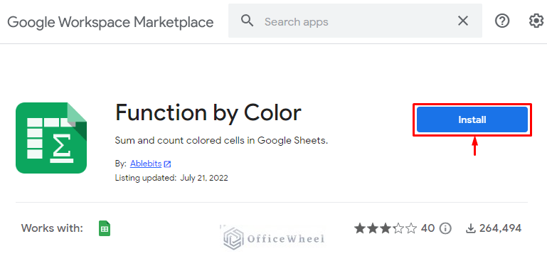
Step 2: In the Marketplace window, search for the Function by Color add-on. Install the one with the highest downloads. See the following image:

During installation, the add-on will ask for permission to access your Google Sheets. Allow it.

You should now have the add-on available under the Extensions tab:

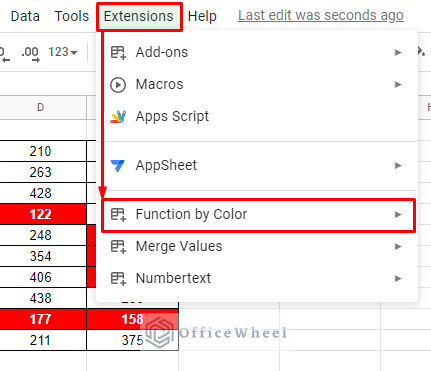
If it doesn’t immediately appear, simply reload the worksheet.

Now, we can take either of the two following approaches to work with the red-colored cells in our worksheet:

I. Using the Add-On Window Feature

As we mentioned before, we will be performing two tasks with cells with the red color in Google Sheets: Sum and Count.

Step 1: Start the Function by Color add-on.

Extensions > Function by Color > Start

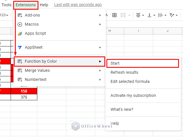
This will open the Function by Color add-on window:

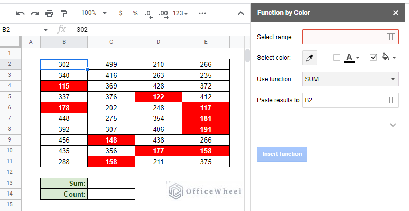
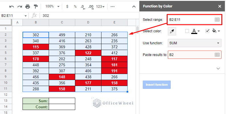
Step 2: Select the data range for the function. You can manually select it using the cell mesh icon on the right of the field. In this case, it is B2:E11.

Step 3: Use the eye-dropper tool in the window to select the cell with a red background color. Important: The color chosen must be within the data range.

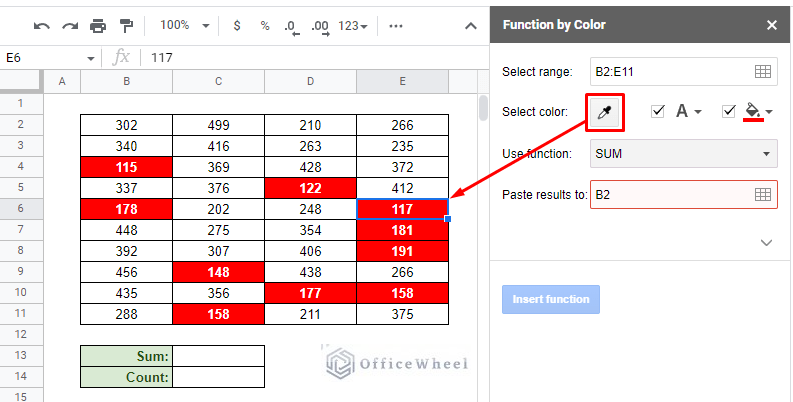
Step 4: There are a lot of functions to choose from, but in this case, we will choose SUM since we want to sum the values in the colored cells.

Step 5: Finally, select the cell you want to paste your results in. In this case, it is C13.

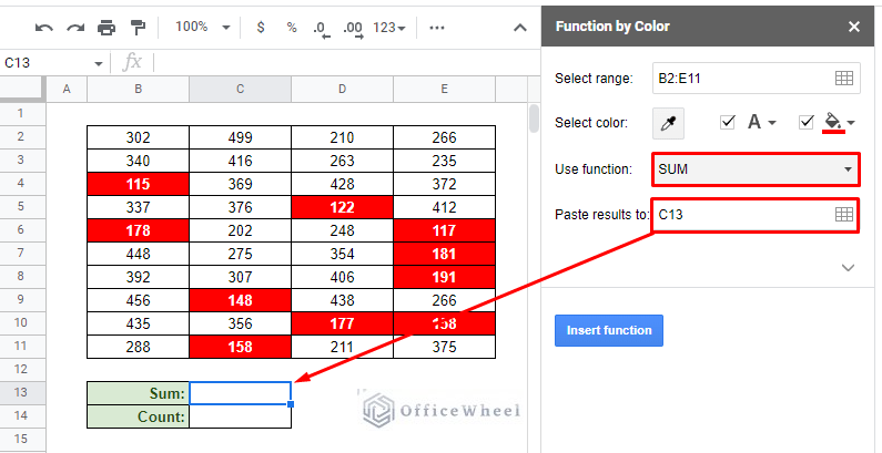
Step 6: Click on the Insert function button to calculate the sum of the cells with the red color background in Google Sheets.

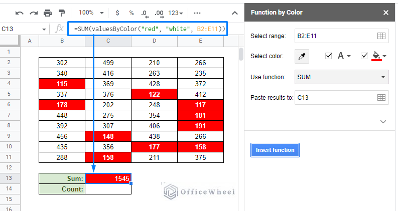
It is important also to note the formula in the formula bar. This is an auto-generated formula for this particular sum with a condition. We will come back to the function VALUESBYCOLOR again later.

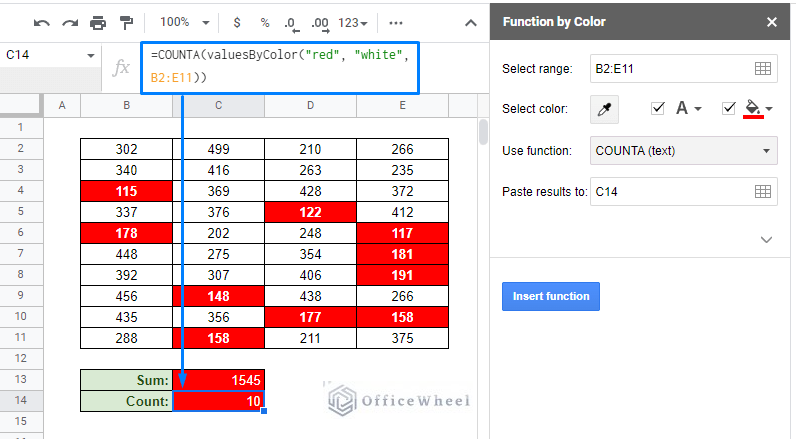
Now, to count the number of cells if the color is red as the background in Google Sheets, simply change the function to COUNTA (text) and set the result location to cell C14:

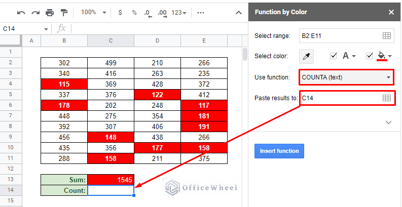
Insert the function again:

II. Using the Functions that Come with the Add-On

Recall the function we asked you to note in the previous section: VALUESBYCOLOR. This is a function that comes with the Function by Color add-on.

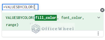
The function returns the values of the cells that match the fill_color and font_color in the range.

The application is quite simple for both summing and counting cells with color:

Step 1: In the desired cell, open the function that you want to perform: SUM for adding values or COUNTA for counting the number of cells. We have chosen SUM in this case.

Tip: If you want to perform VALUESBYCOLOR with conditions, you can also apply functions like SUMIF/SUMIFS or COUNTA/COUNTIF and so on.

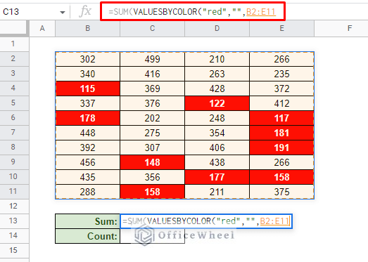
Step 2: Input the parameters of the function. The fill color is “red”. Since we don’t care about the font color, leave it as a blank. The cell range is B2:E11.

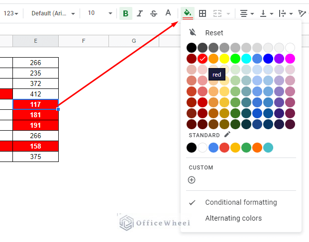
Tip: You can find the fill color name by clicking on the cell and opening the Fill color palette of Google Sheets. The current color will be highlighted with a tick mark.

Step 3: Close parentheses and press ENTER to apply.

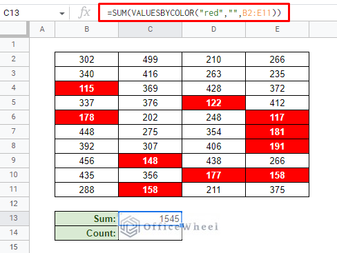
On the other hand, the formula to count the number of cells with the red color in Google Sheets is:

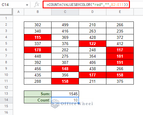
Using the formula directly in the cell not only gives users freedom but also does not allow other features to be applied like the result formatting we have seen in the previous section.

Finally, as a reminder, you must have either the Function by Color or Power Tools add-ons installed to use this function.

2. Use Apps Script to Take Action in Cells that are Red Color in Google Sheets

Add-ons are meant to provide the general users of Google Sheets with a simple way to apply certain functions in the application.

However, if you want a more involved approach and want to try creating your own function to cater to your requirements, Google Sheets has a solution for that too: Apps Script.

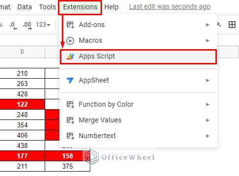
Step 1: Navigate to the Apps Script option from the Extensions tab.

Extensions > Apps Script

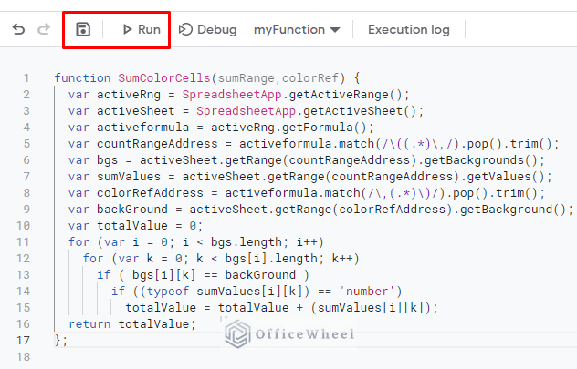
Step 2: Enter the following code to sum all values of cells with the red color in Google Sheets:

function SumColorCells(sumRange,colorRef) {
  var activeRng = SpreadsheetApp.getActiveRange();
  var activeSheet = SpreadsheetApp.getActiveSheet();
  var activeformula = activeRng.getFormula();
  var countRangeAddress = activeformula.match(/\((.*)\,/).pop().trim();
  var bgs = activeSheet.getRange(countRangeAddress).getBackgrounds();
  var sumValues = activeSheet.getRange(countRangeAddress).getValues();  
  var colorRefAddress = activeformula.match(/\,(.*)\)/).pop().trim();
  var backGround = activeSheet.getRange(colorRefAddress).getBackground();
  var totalValue = 0;
  for (var i = 0; i < bgs.length; i++)
    for (var k = 0; k < bgs[i].length; k++)
      if ( bgs[i][k] == backGround )
        if ((typeof sumValues[i][k]) == 'number')
          totalValue = totalValue + (sumValues[i][k]);
  return totalValue;
};

The name of the function is SumColorCells. We will call this function in the worksheet.

Step 3: Save and Run the code. Allow the prompt that asks for access permission.

Step 4: Back in the worksheet, call the SumColorCells function with its two parameters:

• Range: B2:E11 (the data range)
• Background Color: D10 (any cell that has the color in the data range)

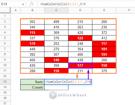
Step 5: Close parentheses and press ENTER to apply. Don’t worry if it takes a few seconds to load.

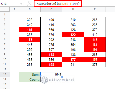
Note: If it’s not working, reload the page and try again.

An In-Depth breakdown of the Script: How to Sum Colored Cells in Google Sheets (2 Ways)

As for counting the number of cells with red color in Google Sheets, the code is:

function CountColorCells(countRange,colorRef) {
  var activeRng = SpreadsheetApp.getActiveRange();
  var activeSheet = SpreadsheetApp.getActiveSheet();
  var activeFormula = activeRng.getFormula();
  
  var countRangeAddress = activeFormula.match(/\((.*)\,/).pop().trim();
  var bgs = activeSheet.getRange(countRangeAddress).getBackgrounds();
  var colorReference = activeFormula.match(/\,(.*)\)/).pop().trim();
  
  var backGround = activeSheet.getRange(colorReference).getBackground();
  var countCells = 0;
  
  for (var i = 0; i < bgs.length; i++)
    for (var k = 0; k < bgs[i].length; k++)
      if ( bgs[i][k] == backGround )
        countCells = countCells + 1;
  return countCells;
};

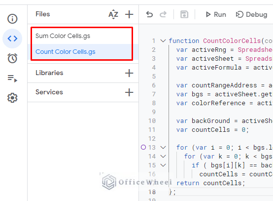
The name of the function is CountColorCells.

Tip: Create separate files for each of the functions.

The result:

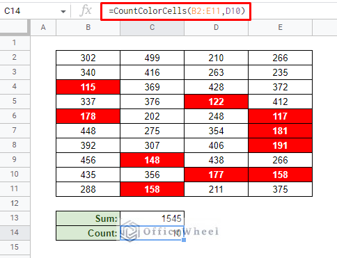
An In-Depth breakdown of the Script: Count Cells with Color in Google Sheets (3 Easy Ways)

Final Words

That concludes all the ways we can use to work with cells if the color is red, or any color for that fact, in Google Sheets.

Feel free to leave any queries or advice you may have for us in the comments section below.

Frequently Asked Questions

• Can you do an IF statement in sheets based on color?

Yes. But with a few extra steps.

Even though great IF statement functions like SUMIF(S) and COUNTIF(S) exist, users cannot include a color condition as a parameter for these functions, simply because there’s no built-in way to do so.

So users have to rely on add-ons like Power Tools or Function by Color or even create their own with Apps Script to get the work done.

• Can an IF statement change cell color?

Yes. We can easily do so by applying conditional formatting to the cells. Even for the most complex IF statements, we can employ custom formulas in conditional formatting.

• Can you apply conditional formatting based on another cell in Google Sheets?

Yes. You can apply conditional formatting on one cell based on the value of another cell in Google Sheets.

This is primarily done with the help of custom formulas in conditional formatting.

Related Articles for Reading

• How to Format Cells to Fit Text in Google Sheets (2 Ways)
• How to Auto Sum in Google Sheets
• Applying SUMIF from Another Sheet in Google Sheets
• COUNTIF Across Multiple Sheets in Google Sheets