Google Sheets: Sum If there are Multiple Conditions (3 Ways)

In this simple tutorial, we will look at a few scenarios where we sum values in Google Sheets if there are multiple conditions.

The Core of the Process: The SUMIF and SUMIFS Function

Adding values with a condition is a common task in Google Sheets. For that, the application has the built-in SUMIF function.

Where:

• range: This is the range where we will look for the condition.
• criterion: The condition we are looking for
• sum_range: The range of cells that will be summed if the condition is positive. If the range and the sum_range is the same, this field is optional.

Here, we have calculated the total customers from Florida:

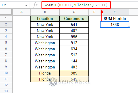
What if we have multiple conditions to sum the values?

For that, we have the SUMIFS function. This works similarly to SUMIF but can take more than one criterion as an argument.

As you can see, the sum_range is not optional here. So, you have to designate a range to sum the values of, even if it falls under a conditional data range.

We will use these core functions depending on different yet common scenarios where we sum values if there are multiple conditions in Google Sheets. Let’s have a look at these.

3 Scenarios to Sum in Google Sheets if there are Multiple Conditions

When we perform a calculation in Google Sheets with multiple conditions, logic is always involved:

1. AND
2. OR

The AND logic is when we want all the conditions to be TRUE before the calculation.

Whereas, the OR logic is when either condition can be TRUE before the calculation is performed.

This gives rise to different scenarios for summing with multiple conditions.

1. Sum if Multiple Conditions are in Different Columns in Google Sheets (AND Logic)

In most common scenarios, you’ll have a dataset with multiple columns that carry data for the conditions:

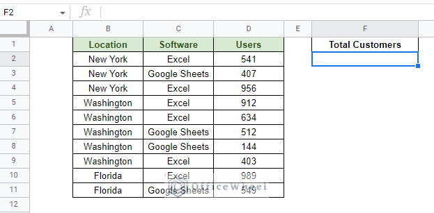
For example, let’s say that we want to find the total number of Users from Washington that use Google Sheets.

Here, both conditions of Washington and Google Sheets must be TRUE for us to sum the total, which means AND logic.

The perfect function for this is SUMIFS since the function says that both conditions must be true before adding the values in the sum_range:

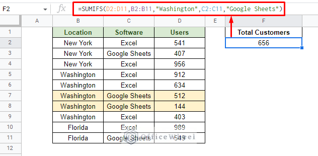
Where:

• D2:D11: Is the sum_range of the dataset.
• B2:B11,”Washington”: Range and condition for the first criterion.
• C2:C11,”Google Sheets”: Range and condition for the second criterion.

Like this, many more conditions can be included in the formula. However, all of them will be in the AND logic.

SUMIFS Error and How to Solve it

In the following image we see a common error faced by users using the SUMIFS function:

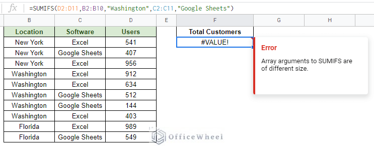
This is because the number of rows in the sum_range argument (D2:D11) does not match the range of one of the criteria (B2:B10):

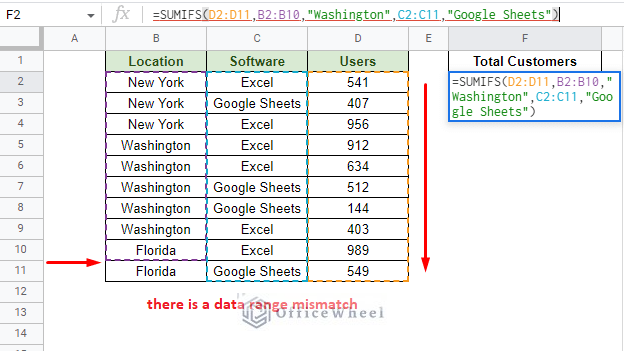
This is a common issue primarily derived from human error.

To solve this, all you have to do is make sure all the ranges involved have the same starting and ending row numbers.

The image above also highlights the ranges applied in the formula. You can visually see where the discrepancy is.

2. Sum if Multiple Conditions are in the Same Column in Google Sheets (OR Logic)

What if we want to find the total number of customers from either New York or Florida?

This is a problem for the OR logic.

This also means that we cannot use the SUMIFS function for this problem, leading us to be more creative with it.

Here, we will use a SUMIF function for each condition. Next, we will add the values using the OR operator (+).

The formula for the “New York” condition:

The formula for the “Florida” condition:

This gives us the final formula::

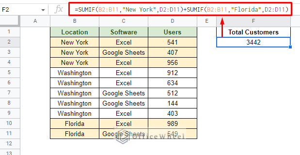
This method is recommended to not be utilized for conditions in multiple columns since there’s a chance of overlapping sum values.

Also check out our article where we use SUMIF(S) with specific and partial text conditions: Find the Sum of Cells with Specific Text in Google Sheets

3. Using ARRAYFORMULA with SUMIF to get Results in an Array for Multiple Conditions

Now, let’s consider a scenario where we have to use both the OR and AND criteria together. For example: Find the total number of customers from New York and Washington that use Google Sheets.

Here we have two conditions:

With AND the best way to go is SUMIFS. And for the two OR conditions, we have to find a match for them using the REGEXMATCH function.

The base formula is:

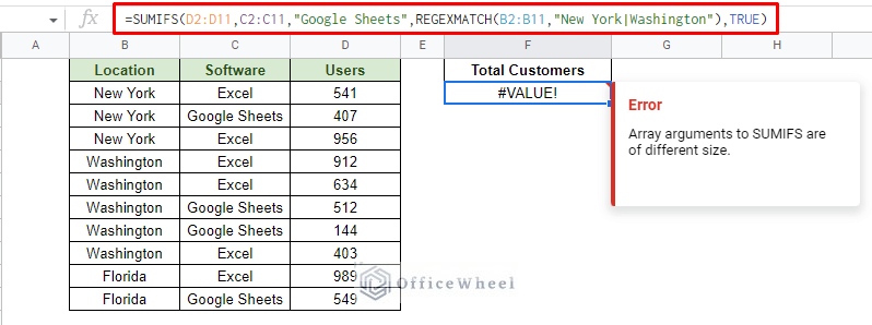
As you can see, we get an error claiming that “the array arguments are of different sizes”.

Here, New York will give us one range of results and Washington another. In Google Sheets, this data will be seen as an array (two separate data) making them have two different sizes.

To remedy that, we have to enclose the formula inside ARRAYFORMULA:

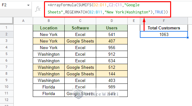
Tip: Press CTRL+SHIFT+ENTER instead of just ENTER at the end of the formula to automatically apply ARRAYFORMULA around it.

Formula Breakdown:

We will start from the center and make our way outwards.

1. REGEXMATCH(B2:B11,”New York|Washington”)

• This is the criterion range, to be more precise the criteria_range2 of the SUMIFS function.
• The REGEXMATCH function checks the range B2:B11 for either New York or Washington.
• The pipe symbol (|) acts as the OR condition in this case and for the whole formula.

2. REGEXMATCH(…),TRUE

• The TRUE statement is essentially the criterion2 argument of the SUMIFS function.
• If REGEXMATCH returns TRUE after a match is found, this TRUE will signal the SUMIFS function to count that cell in the sum_range argument.

3. C2:C11,”Google Sheets”

• The range and condition for the first criterion. No complexity here.

4. D2:D11

• The sum_range of the SUMIFS function.

Final Words

That concludes our simple tutorial for how to sum in Google Sheets if there are multiple conditions.

While the SUMIF(S) function serves as the core, understanding which multiple criteria logic (AND or OR) is needed will change how you can approach the problem.

Feel free to leave any queries or advice you might have for us in the comments section below.

Related Articles for Reading

• Google Sheets: Sum an Entire Column (4 Easy Ways)
• How to Auto Sum in Google Sheets
• How to Perform Conditional Sum in Google Sheets (Easy Guide)
• Applying SUMIF from Another Sheet in Google Sheets
• How to Sum Multiple Rows in Google Sheets (3 Ways)