Adding or summing values in a spreadsheet is a common process. And with such a versatile application like Google Sheets, we have so many ways we can use to sum an entire column of values in a spreadsheet.
From the built-in Status Bar to direct view results to simple functions that users can customize their calculations, Google Sheets has it all.
But, to keep things simple, and considering common scenarios that most users face, we’ve kept the number of methods to four. Each adding something new catered to their respective situations.
Let’s get started.
4 Ways to Sum an Entire Column in Google Sheets
1. Directly View the Sum of an Entire Column right in the Google Sheets Window
Summing is a fundamental yet simple calculation. We all know how to do it automatically and so does Google Sheets.
For simple calculations like Sum, Google Sheets has the Status Bar at the bottom-right of the window that appears when you select cells in the worksheet.
For example, let’s say we have the following worksheet:
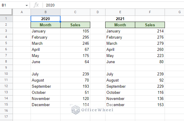
We have a common scenario of Sales values by Month and Year. There is also a split depicting the first and second halves of the year.
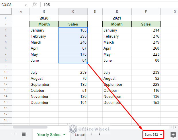
Let’s say we want to find the total Sales value of 2020.
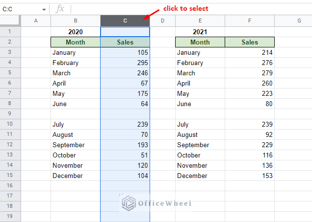
All we have to do is click the column number of the Sales column, in this case, it is column C:
And take a look at the bottom-right of the Google Sheets window:
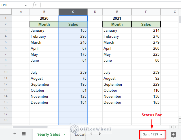
This is the Status Bar that shows the sum of the entire selected column in Google Sheets.
Google Sheets has preemptively guessed the user’s intentions and added all the numerical values of the selected column to present the sum.
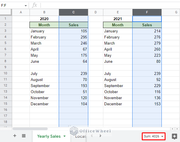
This can work for multiple selected columns:
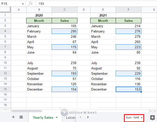
Any selected range of cells in the worksheet:
Or any selected cells, period.
This is a great way to view primary calculations, especially if you don’t want to dedicate cells for this in the worksheet. This can work for other reasons like quick viewing calculations and reluctance to change the format of the existing worksheet.
Clicking on the Status Bar will show you the results of other calculations that Google Sheets has done in the background:
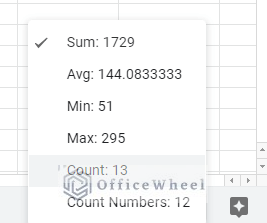
Of which the Average (Avg) is another important one in any spreadsheet.
2. To Sum in Google Sheets Directly from the Toolbar
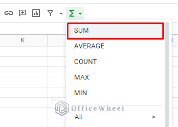
Another useful feature that Google Sheets has for its users is the Functions menu right in the toolbar:
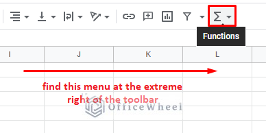
This menu has a list of all the functions available in the application. While it may sound overwhelming, Google Sheets groups all the common functions like SUM up at the top of the list.
While accessing the function may be easy, working with them in this way may be a little clunky. Let’s show you what we mean:
If we want to sum an entire column, we must first select the column and then apply the SUM function, and this time, from the Functions menu.
See what happens when we do this:
There are 3 things going on here:
- A function must occupy a cell in the worksheet to present the results.
- The application of any function with the Functions menu will make Google Sheets automatically set the result location.
- The result location is usually an adjacent cell or a part of the selected cells.
With these points in mind, we can understand that the user has no control over where the result will go!
To work with this method, we cannot select the entire column, but select only the range of cells that we actually need:
Select range of cells > Functions > Sum
To conclude, this method should only be used when you have a simple arrangement of data.
In the next section, we solve this issue by directly applying the SUM function according to the user’s choice.
3. Use the SUM Function to Sum an Entire Column
Why not take back some control from Google Sheets this time?
We are talking about applying the SUM function ourselves.
If you don’t already know, the SUM function is one of the fundamental functions you’ll learn in Google Sheets.
SUM(value1, [value2, ...])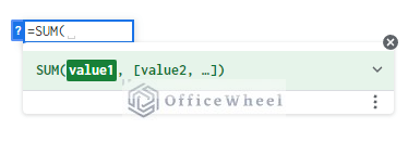
The function can take multiple ranges of cells at once to do a single task: Addition.
Here we have a sample dataset containing Location and Customer data. We want to find the total number of customers:
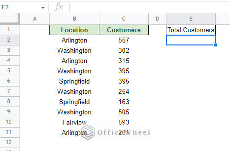
To sum up the entire Customers column in Google Sheets, simply open the SUM function, =SUM(, and click on the column number to select the entire column range.
Close parentheses and press ENTER.
=SUM(C:C)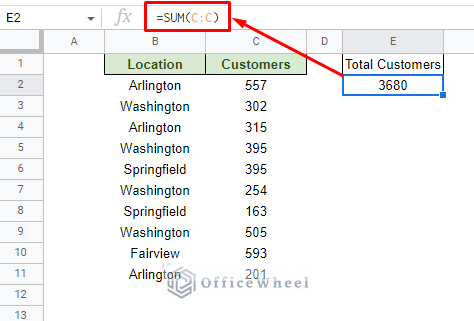
The advantage here above the previous method is that we can set the location of the result ourselves.
Setting the range up like this, C:C, includes all the cells in column C.
The advantage of this is that it makes the formula dynamic to the column. Meaning, every time we enter a new value into the column, it will be added to the total sum:
But, if you want a limited range of only a few cells in the column, simply update the range in the formula.
=SUM(C2:C11)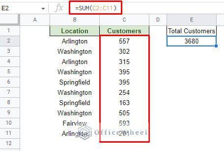
This version is much more common.
Extra: Sum Different Ranges from Different Columns in Google Sheets
Recall the SUM function syntax. Using this function, we can sum multiple different cell ranges that don’t always have to be adjacent.
That means, we can do something like finding the total sales of the first and last quarters of the years 2020 and 2021 from the previous worksheet:
=SUM(C3:C5,C13:C15,F3:F5,F13:F15)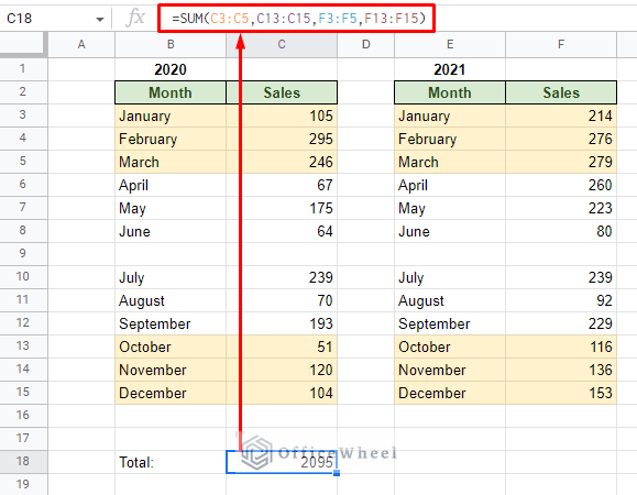
Each non-adjacent range is separated by a comma, highlighted in the image above in yellow.
4. Add Column Values with Criteria Using SUMIF or SUMIFS functions
We can’t really call it a sum process in a spreadsheet without adding in a few conditions, can we?
Adding values in Google Sheets is quite easy with the SUMIF function.
SUMIF(range, criterion, [sum_range])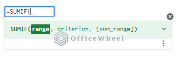
The function takes a range of cells upon which a criterion is applied. We can either sum the values in the range or apply a separate “sum range” from where we will get our result.
For example, we have the following worksheet from where we want to find the total number of customers that have gone to a location with a rating of more than 5:
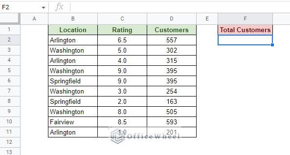
The formula will be:
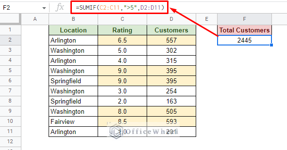
Where:
- C2:C11 is the range of values for the Rating column. Here, the “>5” criterion is considered.
- D2:D11 is the range of the column whose values will be added if they meet the criterion.
Why not add another condition to the mix?
Let’s say we also want to know only the number of customers from the Washington region with a rating higher than 5.
While SUMIF can only have one criterion, the SUMIFS function can take multiple.
SUMIFS(sum_range, criteria_range1, criterion1, [criteria_range2, criterion2, ...])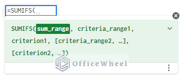
The formula:
=SUMIFS(D2:D11,C2:C11,">5",B2:B11,"Washington")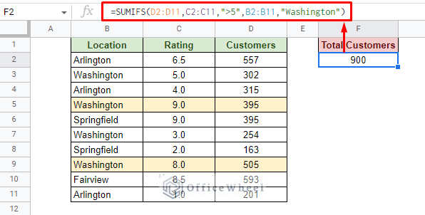
Where:
- D2:D11 is the range of cells that will be summed. The Customers column.
- C2:C11,”>5″: Condition set for the Rating column.
- B2:B11,”Washington”: Condition set for the Location column.
Note: In both cases, SUMIF and SUMIFS, you can remove the bottom row number limitation to make the formula more dynamic and accepting of new values, e.g., D2:D11 to D2:D.
Learn more: How to Perform Conditional Sum in Google Sheets (Easy Guide)
Final Words
That concludes our simple tutorial on how to sum an entire column in Google Sheets.
Each method is best used in specific scenarios and can also depend somewhat on user knowledge. We hope that we’ve been able to clarify these scenarios and you are now well-equipped to use all of these approaches.
Feel free to leave any queries or advice you might have in the comments section below.