How to Sum Cells from Different Sheets in Google Sheets (3 Easy Ways)

In this simple tutorial, we will look at a few ways we can use to sum cells across different sheets in Google Sheets.

While the idea is simple, proper cell referencing plays a huge part as we use different functions for different scenarios.

Let’s get started.

3 Scenarios to Sum Cells from Different Sheets in Google Sheets

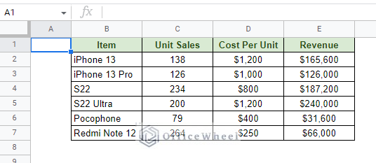
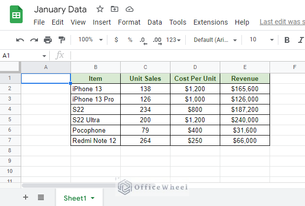
We will use the following datasets spread across multiple worksheets to show our examples. Each contains monthly Sales data for January, February, and March.

For January:

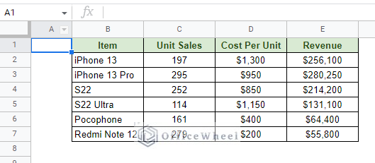
For February:

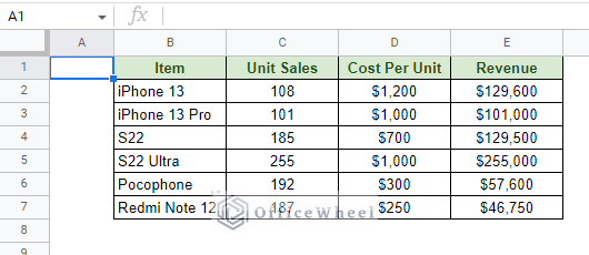
And finally, for March:

Now, we will discuss three separate scenarios where we use these datasets to sum values in Google Sheets.

1. The Basic Sum of Cells Across Multiple Sheets in the Same Google Sheets Spreadsheet

Let’s go to our fourth worksheet that contains (for now) a lone field that wants the total revenue accrued across the months.

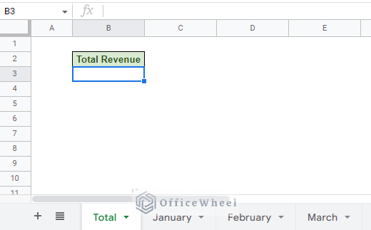
This essentially means that we have to sum the revenue columns of all three months in this field.

And what better way to do this than by using the SUM function?

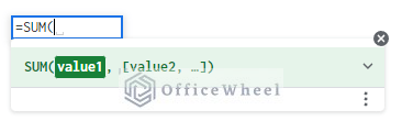
Let’s test it out by summing the total revenue of January:

Step 1: Open the SUM function in a cell, =SUM(.

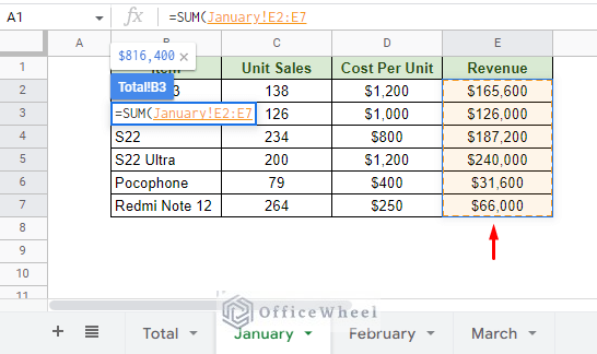
Step 2: Move to the January worksheet and select the revenue range.

The cell reference to a different worksheet in Google Sheets is always in this format:

Step 3: Close parentheses and press ENTER.

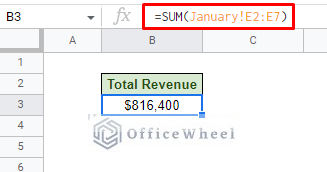
More than simplicity, you will notice that the SUM function can take multiple sum ranges as arguments, making it perfect to reference different sheets to sum in Google Sheets.

So, to calculate the total revenue, we simply have to insert the range of each respective month’s revenue ranges in this formula, separated by commas of course:

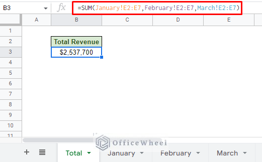
Sum of Cells from Different Spreadsheets in Google Sheets

Being completely browser-based, Google Sheets has a different approach when referencing cells in completely different worksheets. This is done solely on the back of the IMPORTRANGE function.

This function will help reference a cell or a cell range from a different spreadsheet that will be used in the SUM function.

For this example, we’ve placed the Monthly Revenue data in different spreadsheets like this one:

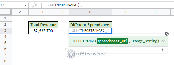
Let’s see how we can sum all the revenues in different spreadsheets:

Step 1: Open the SUM and IMPORTRANGE functions, =SUM(IMPORTRANGE(.

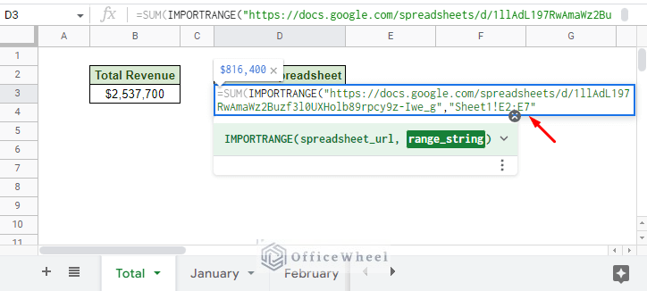
Step 2: For the spreadsheet_url, move to the spreadsheet that contains the data (in this case, it is the January Data spreadsheet) and copy the URL. See the image below:

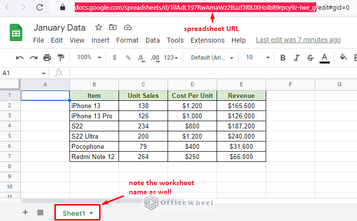
Note the worksheet name as well.

Step 3: Paste the URL inside quotation marks (“”) in the spreasheet_url field. The quotation is important.

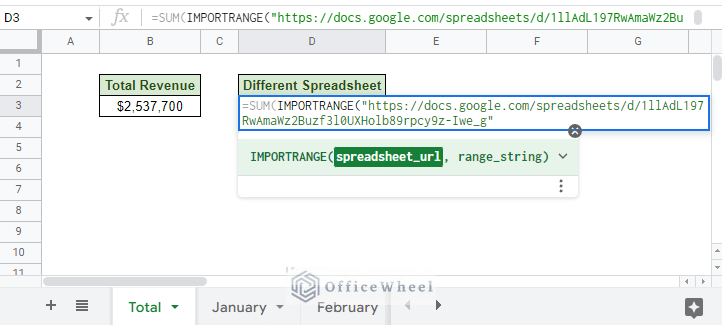
Step 4: For the range_string field, simply enter the worksheet cell range (sheet_name!cell_range) inside quotations (“”) as well.

Remember we asked you to note the worksheet name of the dataset? This is where you’ll use it:

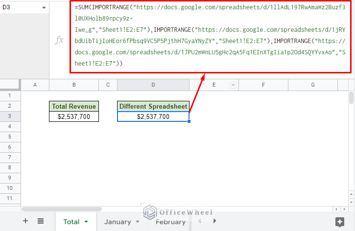
Step 5: Close parentheses and do the same for the other spreadsheets (February and March). The final formula will look something like this:

Important Note: When doing this for the first time, the cell may show a REF error. Simply click on the cell and allow permission to access the other spreadsheets. You may have to do this multiple times depending on the number of referenced spreadsheets.

2. Conditionally Sum Cells from Different Sheets in Google Sheets

Summing with conditions or criteria is a common occurrence in a spreadsheet.

Thankfully, Google Sheets provides its users with a quick and easy way to do so and also allows for the conditions and values to be imported from many different worksheets.

And it all revolves around the SUMIF function.

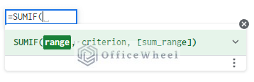
While the final field of the function is given as optional, we will still have to utilize it in this situation.

To sum cells from different sheets in Google Sheets is essentially summing with multiple criteria with each worksheet being a different criterion in this case.

And since any state can work regardless of being present or not, this logic takes the form of the OR condition. This means that we can simply add the SUMIF results of each sheet together to get the total.

For example, let’s say we want to find the total revenue of the item “S22” over the three months. The SUMIF functions for each will be:

January:

February:

March:

The final formula is:

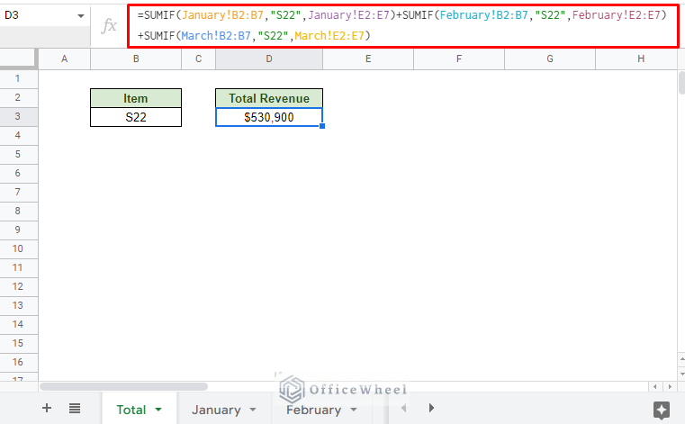
We can update the criterion text for each SUMIF function to point to a single cell reference to make the formula more dynamic:

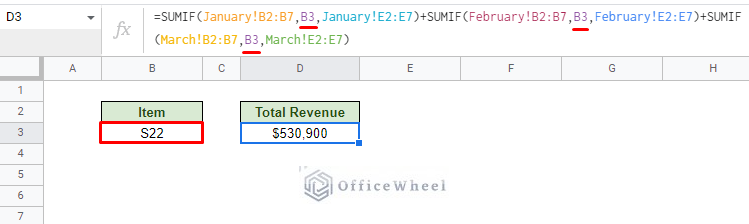
This also gives us a chance to apply a drop-down list to cycle through different items:

Alternatively, the SUMIFS function can also be used here, albeit with different argument locations:

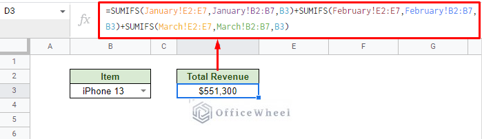
This is best used when you have multiple criteria in the same dataset (AND logic) to look for.

Learn More: Applying SUMIF from Another Sheet in Google Sheets

3. Sum the Same Cell Across Different Sheets in Google Sheets

For all the different Month worksheets (January, February, and March) the Revenue cell for each item is the same. This gives us the advantage of simply referencing the same cell number for each worksheet in the sum.

For example, cell E2 for the iPhone Revenue for each month.

If you’ve used MS Excel or come from it, you may know that you can use the SUM function with a worksheet range if summing the same cell in each worksheet.

However, this is not possible in Google Sheets.

Forcing us to stick to traditional cell referencing to sum the same cells from different sheets in Google Sheets:

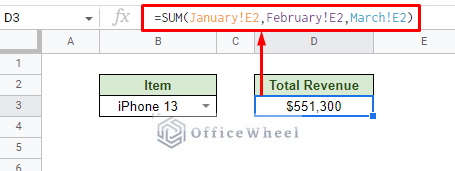
But, if you really want to replicate Excel’s capability of summing the same cell over different worksheets, you have to employ the use of the addon 3D Reference.

Using 3D Reference Add-on to Sum the Same Cell in Different Worksheets

From the add-ons Marketplace (Extensions > Add-ons > Get add-ons) find and install the 3D References add-on.

This will add a new and unique function in Google Sheets called DDDREF.

The function takes the names of the starting and ending worksheets and returns the reference of the given cell or range of cells.

To find the sum of the same cell in different worksheets in Google Sheets, the formula will be:

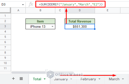
Final Words

That concludes all the ways we can use to sum cells from different sheets in Google Sheets.

With functions like SUM and conditional ones like SUMIF and SUMIFS, there really is no simpler way to work around this topic. All you have to do is make sure the referencing data is correct in each case.

Feel free to leave any queries or advice you may have in the comments section below.

Related Articles for Reading

• How to Add Up A Column in Google Sheets
• How to Sum Multiple Rows in Google Sheets (3 Ways)
• Google Sheets: Sum If Checked (2 Ways)
• Find the Sum of Cells with Specific Text in Google Sheets
• How to Sum Colored Cells in Google Sheets (2 Ways)