How to Use SUMIF in Google Sheets (With Examples)

SUMIF in Google Sheets is one of the core functions in the spreadsheet software. Its application is numerous, of which we will be seeing more of in this article.

Our aim for this article is to make it serve as a go-to page for all your SUMIF needs.

SUMIF Basics: What Does the Function Do?

As the name suggests, the SUMIF function takes the process of the SUM function and adds the IF condition to it.

The syntax:

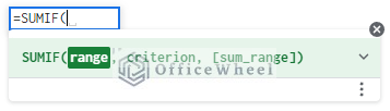
• range: the range of cells to check for criterion.
• criterion: The test or condition to check. It should be, by default, a string.
• [sum_range]: Optional. The range of cells that will be included in the sum. If left blank, it will consider the range field to sum.

As we can understand, the SUMIF function scans a range of cells and sums the values within the range (unless a separate sum_range is defined) according to a condition or criterion.

Note that SUMIF only takes a single IF condition or criterion. For multiple criteria, there exists the convenient SUMIFS function or you can jump to Example 7 of this article for a quick alternative with the SUMIF function.

7 Examples Using SUMIF in Google Sheets

1. Text Match With SUMIF in Google Sheets (Exact Match)

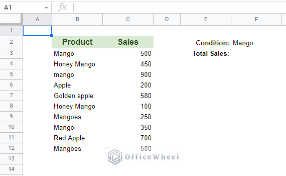
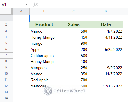
We start with something simple, like calculating the total sales of a given product (e.g. Mango) from the following dataset.

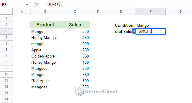
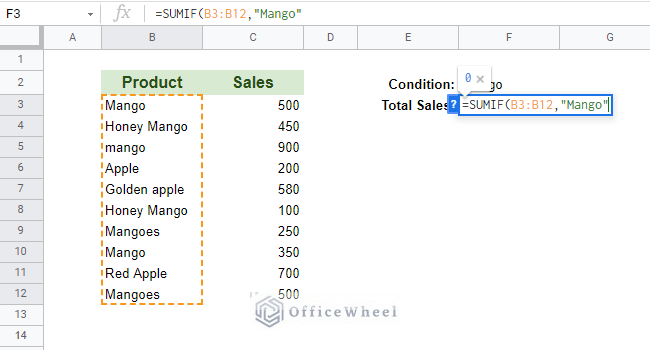
Step 1: Open the SUMIF formula in your desired sell, =SUMIF(

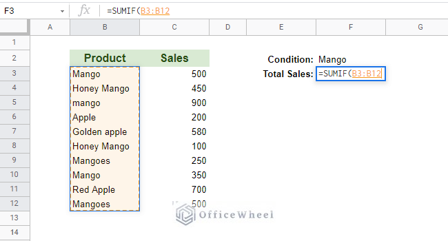
Step 2: Select the range. You can click and drag over the cells. Our range is B3:B12.

Step 3: Input the criterion. Our criterion is the text “Mango”. Since SUMIF only takes strings as conditions, make sure to add quotation marks (“”).

Step 4: Input the sum_range. For us, it is C3:C12 since our Sales information is in a different column.

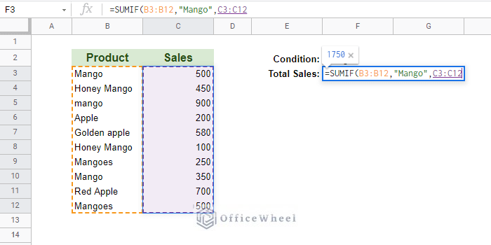
Step 5: Close parentheses and press ENTER.

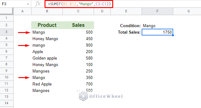
As you have noticed, our formula takes into account only three instances of “Mango” when there are many in the list. This is because SUMIF only takes exact matches of text regardless of the case.

For partial and case-sensitive matches, look to the next two examples.

But before that, we have to mention that you can also use a cell reference for your SUMIF criterion. Our new formula:

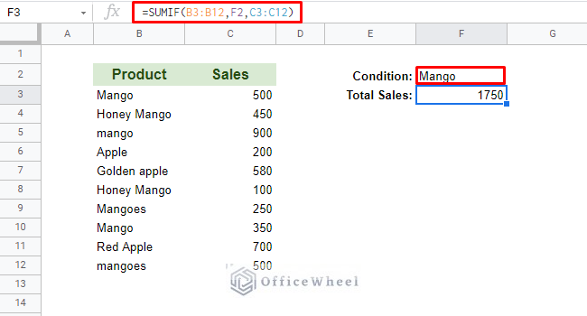
Recall that SUMIF only takes string values as its criterion, and our cell reference only contains a string.

2. Partial Text Match With SUMIF (Wildcards)

It is more than likely that in a practical scenario your dataset may not have neatly organized text. Your search keyword may be coupled with another string in the cell, as we have seen in our last example.

To remedy that, we have to do a partial search. And we can do that by applying wildcards, namely the asterisk (*).

Step 1: Open the SUMIF function and select the range, B3:B12.

Step 2: It is in our criterion section where we see our change from the previous formula. Our criterion this time will be “*mango*”.

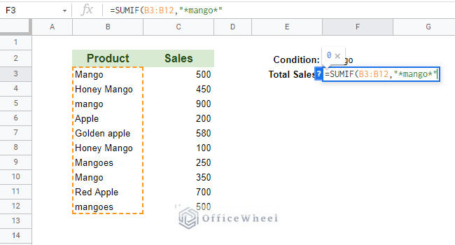
Step 3: Select the sum_range, C3:C12. Close parentheses and press ENTER.

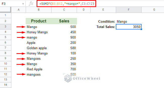
With this formula, all seven instances of “mango” are taken into account, regardless of their case or position in the cells.

This is because the asterisks on either side of our keyword enable the formula to take string values on either side of it.

However, we must be careful about the cell reference version of this formula.

While the word “mango” can be referenced from a different cell, the asterisk (*) symbols can’t be. So we have to add them separately in our condition using quotation marks (“”) and concatenate them to the cell reference with an ampersand (&).

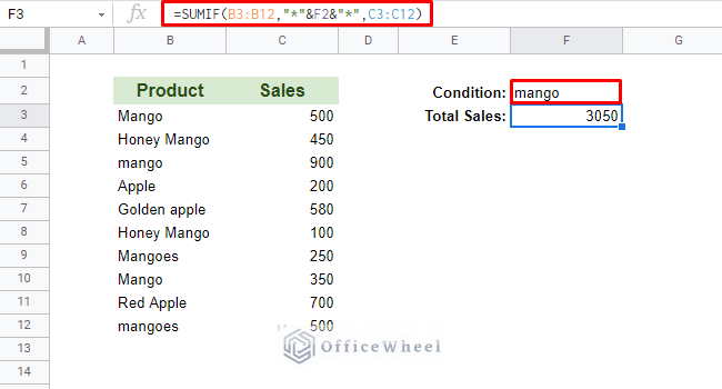
If your range selection contains a wildcard, like an asterisk (*) or question (?), simply add the tilde (~) symbol before the condition: “~*” or “~?”

Formula example:

3. Case-Sensitive Match With SUMIF in Google Sheets

Next, we will look at case-sensitive text conditions for our SUMIF formula. The SUMIF function is not case-sensitive by default, but we can take the assistance of other functions that are to make our search and match case-sensitive.

The two additional functions we are going to use are the FIND and ARRAYFORMULA functions.

We use the same dataset and criteria as before: calculate the total sales of “Mango” from the list. Notice we have only mentioned mango with a capital “M”.

Our formula:

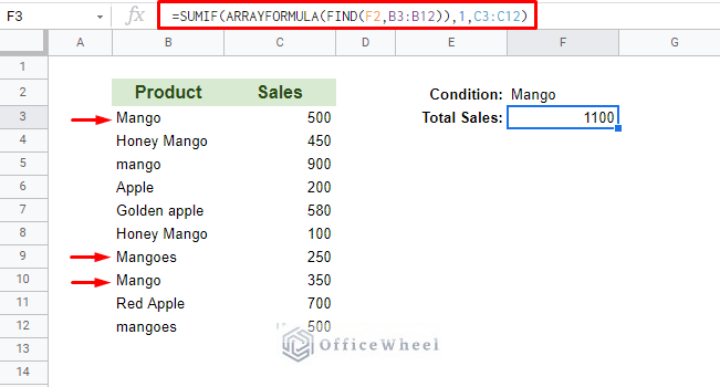
Takes into account all cells that start with Mango

Formula Breakdown:

• FIND(F2,B3:B12)): The FIND function searches for all instances of “Mango” from cell F2.
  • FIND is case-sensitive.
  • FIND searches the string from the start of the cell. Thus Mangoes (row 9) is also included in our sum.
  • FIND only searches in a single cell. Since we gave a range, the function will return an array of values.
• ARRAYFORMULA(FIND(F2,B3:B12)): This is our range section of SUMIF. The FIND function is nested in it. ARRAYFORMULA is required as the FIND formula is returning an array of values.
• 1: Our value of criterion. Also depicts Boolean TRUE. The FIND formula returns TRUE for the matches, thus 1 is the condition to sum.
• C3:C12: Our sum_range.

4. SUMIF With Number Conditions

Next up we have number conditions for our SUMIF function.

We have four number conditions:

1. Greater than
2. Less than
3. Equal to
4. Not equal to

For Greater than and Less than, the symbols will suffice.

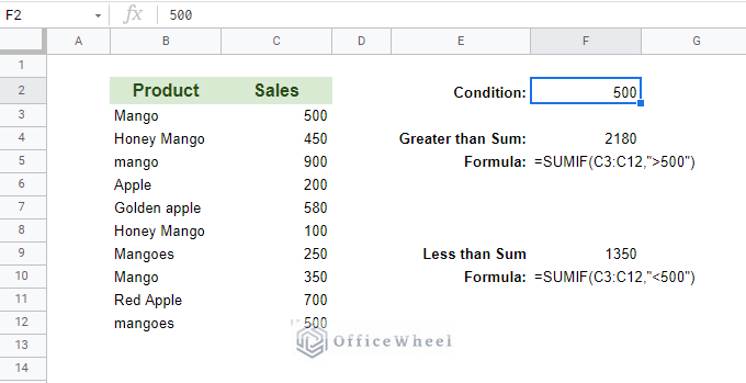
Greater than SUMIF formula:

Less than SUMIF formula:

Points to Note:

• We have not included the sum_range section as it is covered by the range.
• We can add an equal-to symbol (=) to the condition to make Greater than and equal-to (>=) or Less than and equal-to (<=) conditions.

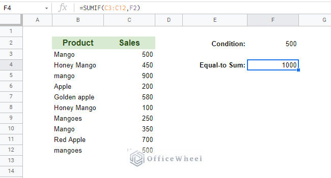
For an Equal-to condition, you can simply write the number or present it like this, “=500”.

Equal-to SUMIF formula:

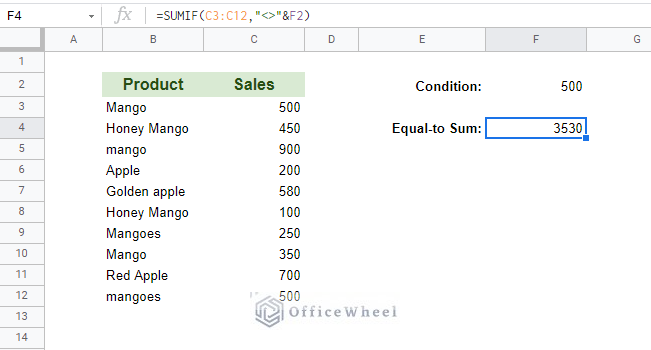
For the Not equal-to condition, we simply use the not equal-to symbol (<>).

Our formula:

5. SUMIF With Dates in Google Sheets

Dates in Google Sheets are seen as numbers. Meaning, we can treat conditions for dates the same way as we did for numbers in our previous method.

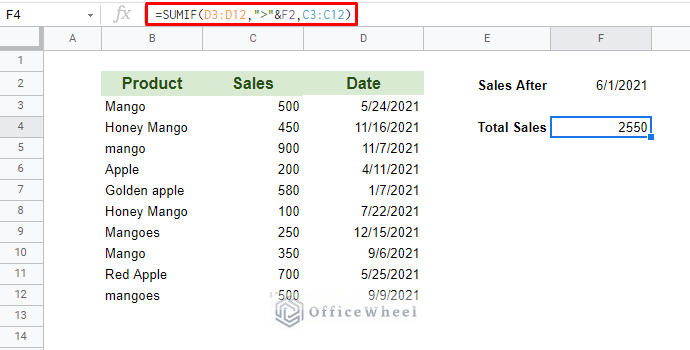
So, if we want to calculate the total sales of products from the 1st of June 2021, our SUMIF formula can be written as:

You can also implement date functions of Google Sheets into the formula like DATE and TODAY.

SUMIF with DATE function:

As you have noticed, it is the criterion section that needs to be changed every time. For example, we can replace DATE(2021,6,1) with TODAY() to find and sum all occurrences that happen starting tomorrow.

6. SUMIF Conditions With Blank and Non-Blank Cells

Now let’s consider a scenario where we have some missing dates in our dataset.

Our SUMIF condition this time will be to calculate the total Sales of Products, once for those who have Dates (non-blank cells) and another for those that don’t have Dates (blank cells).

SUMIF formula for blank cell condition:

Note: You can use “=” as a condition instead, to also ignore whitespaces.

SUMIF formula for non-blank cell condition:

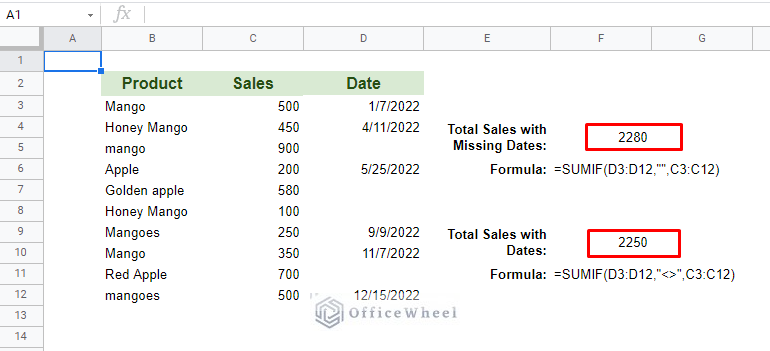
7. SUMIF With Multiple Criteria Using OR Logic

Trying to find outputs based on multiple criteria is a very common occurrence in spreadsheets.

With SUMIF, it is possible only by adding multiple SUMIF formulas together. This is also known as the OR logic.

On our existing dataset, let’s say we want to find the total Sales of both “mango” and “apple” conditions (we are keeping things simple).

The formula to find the total sales of “mango”:

The formula to find the total sales of “apple”:

Combined SUMIF formula with OR logic:

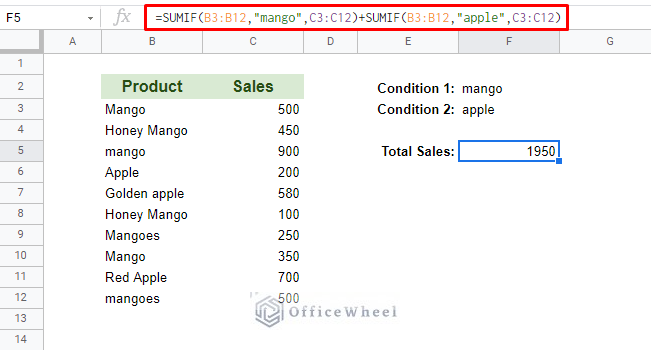
Note: Of course, there is an AND logic version of SUMIF with multiple criteria, but that is better utilized with the SUMIFS function.

Final Words

We hope that this article has given you a better insight into the SUMIF function of Google Sheets, which is one of the core functions of any spreadsheet application.

Please feel free to leave a comment on any queries or advice you might have for us.

Related Articles for Reading

• Applying SUMIF from Another Sheet in Google Sheets
• How to Perform Conditional Sum in Google Sheets (Easy Guide)
• Google Sheets: Sum If Checked (2 Ways)
• How to Add Up A Column in Google Sheets
• How to Sum Multiple Rows in Google Sheets (3 Ways)