How to Compare Text in Google Sheets (3 Easy Ways)

Today, we have a look at a few ways we can use to compare text in Google Sheets.

Let’s get started.

3 Ways to Compare Text in Google Sheets

1. Using the Comparison Operator

The fundamental way to compare anything in Google Sheets, including text, is by using the comparison operator or equals-to symbol (=).

This symbol checks two cells for a match of the contents. Let’s see it in action:

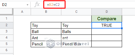
The result we get is in Boolean (TRUE or FALSE).

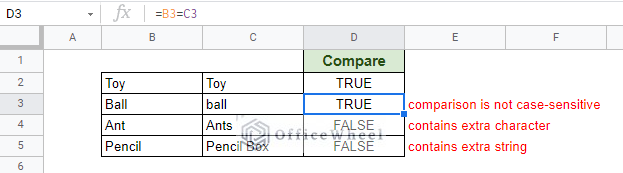
Note that we have mentioned a match, meaning that while this comparison is not case sensitive, other conditions must be the same.

For the comparison to return TRUE:

• The values will not contain extra characters along with the matching string.
• Extra text should not be present.

2. Using the EXACT Function to Compare Text in Google Sheets

The EXACT function, as the name suggests, makes a one-to-one comparison of two cells, whether it be text or numbers.

The EXACT function syntax:

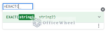
The main difference between the EXACT function and the comparison operator is that the function makes no compromises when comparing, even for the text case.

The EXACT function in action:

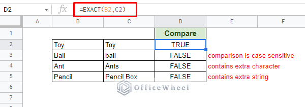
Return a Meaningful Message With IF Function

While a Boolean value gives a concrete result, it is not that meaningful when presenting it as data in a presentation or a report.

To take this value and return a meaningful message, we can utilize the IF function. The IF function allows us to take the Boolean values and attach a text message to the results.

Our formula:

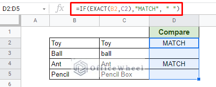
On a side note, we can also use conditional formatting to highlight matching text in Google Sheets. The conditional formatting will take the boolean values of the base formula.

3. Compare a Combination of Text

So far, we have tried to compare text to get a match of a single value in Google Sheets. While it can get most of the work done, in many cases, however, you may need to find a match for a combination of text.

There is no simple way to approach it. We have to resort to a combination of formula and logic to solve this problem.

Here we have two cells that contain the same combination of three words.

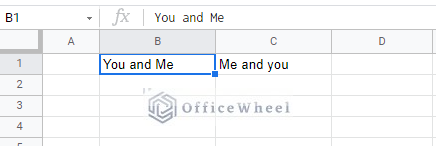
Our target is to show whether both cells have the exact text no matter their position in the cell. Let’s go about it step-by-step.

Steps to Compare a Combination of Text

Step 1: Split the text in one of the cells to make it easier to compare. We use the SPLIT function.

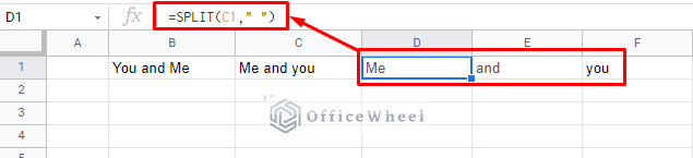
Step 2: Check with cell B1 for a match. We use the SEARCH function for this. It will return the position of the matched text as numbers.

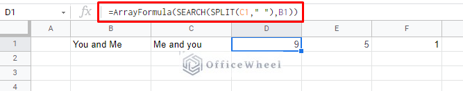
Since we have multiple words, we will get multiple numbers. To view all of them we have to apply ARRAYFORMULA.

Note that if there is no match, we will get an error.

Step 3: We do the same for the other cell. Switch B1 and C1 for this formula.

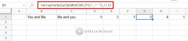
Step 4: We combine the two functions.

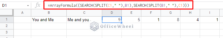
Step 5: We will now use the IFERROR function to overcome the error that we might get during a mismatch.

We will see the significance of the “1000” as the error return in the next step.

Step 6: Logic states that if we get a complete match, the formula will return a number (position). Thus, we can SUM these positional values to act as a condition for our comparison.

Since our string does not contain more than 3 words, it is safe to say that the sum will not exceed 100. If it does, it will only be in the case of a mismatch or an error, since the IFERROR will return the value 1000 for every mismatch.

We will implement an IF function to return TRUE for a match or FALSE for a mismatch to round off our conditions.

Our formula:

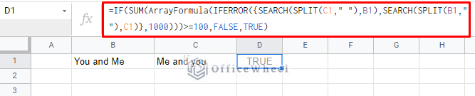
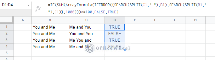
Applying to other text combinations:

Final Words

That concludes all the ways we can compare text in Google Sheets. We hope that our discussion comes in handy for your tasks.

Please feel free to leave any queries or advice you might have in the comments section below.

Related Articles for Reading

• Compare Two Columns in Google Sheets (5 Easy Ways)
• Using Conditional Format to Compare Two Columns in Google Sheets
• Compare Two Columns for Duplicates in Google Sheets (3 Easy Ways)