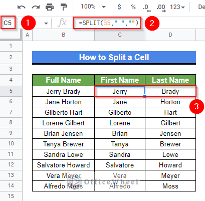
We often require to split appended values from a cell. For example, we may want to separate URLs and email extensions or extract known values from a string. Here, I’ll demonstrate 9 quick methods to split a cell in Google Sheets. Here is an overview of our required result. We have used the SPLIT function to separate a cell around the Space (“ ”) delimiter.
A Sample of Practice Spreadsheet
You can copy our practice spreadsheets by clicking on the following link. The spreadsheet contains an overview of the datasheet and an outline of the demonstrated examples to split a cell in Google Sheets.
9 Quick Methods to Split a Cell in Google Sheets
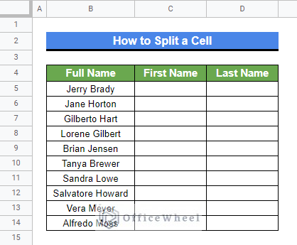
First, let’s look at the dataset we’ll use for most of this article. The dataset contains a list of names that we want to split into two different cells. Now, let’s get started.
1. Using Split Text to Columns Feature
To start, let’s split the required cells without applying any formula. We can use the Split Text to Columns feature to separate values around a single delimiter. There are two ways to apply the Split Text to Columns feature as described in the sections below.
1.1 Applying from Clipboard Menu
First, we’ll apply the Split Text to Column feature from the clipboard menu options. The clipboard menu is generated while applying the Paste command. And then the Split Text to Columns command can put the space-separated values into different columns.
Steps:
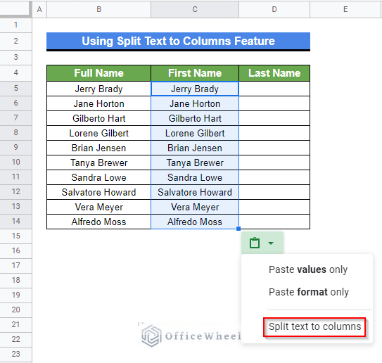
- Afterward, select Cell C5 and paste the range using the keyboard shortcut CTRL+V. At this time, the clipboard for paste formatting will be visible. Click on the Clipboard menu.
- As soon as you click on the Clipboard menu, a list of options will appear. Select the Split Text to Columns feature from the list.
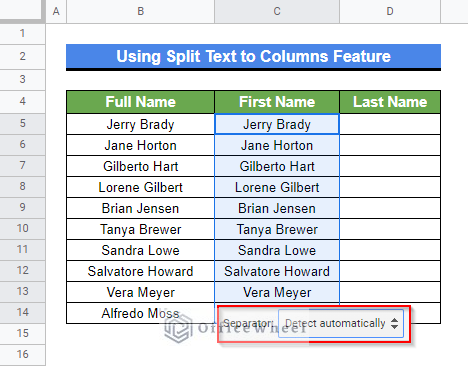
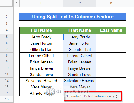
- At this time, a new clipboard will appear, where you can select the separator to execute the Split Text to Columns feature. Click on the Separator clipboard.
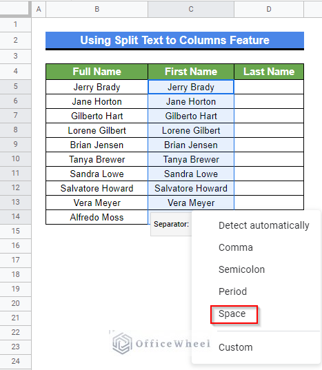
- A list of separators will be visible now. We’ll select the Space option from here. You can choose the separator you require. You can also insert a custom separator if it isn’t available in the appeared list.
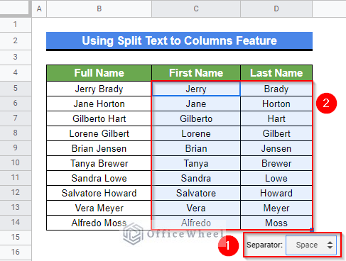
- As soon as you select the Space option as the separator for the Split Text to Columns command, the copied values will be split into required columns.
1.2 Implementing from Data Ribbon
In lieu of using the clipboard menu, we can also perform the Split Text to Columns command from the Data ribbon. Keep reading to learn how.
Steps:
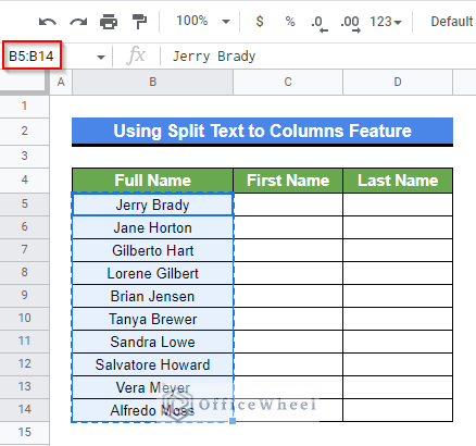
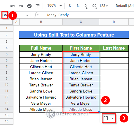
- Follow the first two steps of the previous method to copy and paste the range B5:B14 to C5:C14 by using the Ctrl+C and Ctrl+V keyboard shortcuts.
- Then, select the range C5:C14 and go to the Data ribbon.
- From the appeared options, select Split Text to Columns feature.
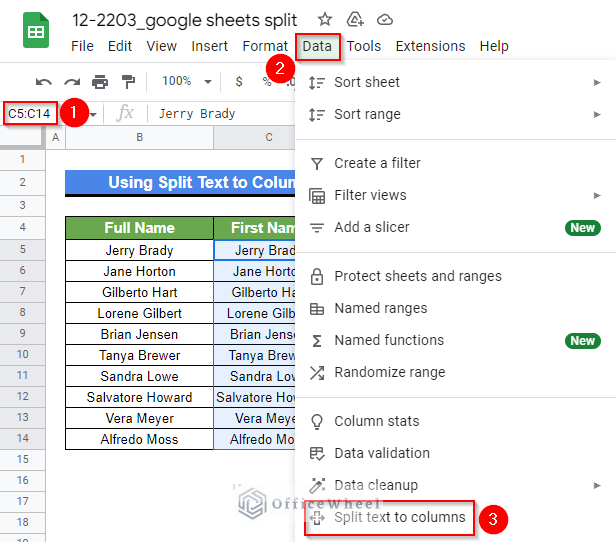
- A clipboard will appear at this time, where you can select the separator to execute the Split Text to Columns feature.
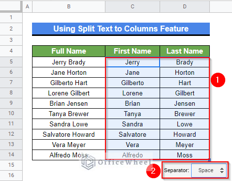
- A list of separators will be visible when you click on the Separator clipboard. We’ll select Space as a separator from there. This will provide us with the required result like the following.
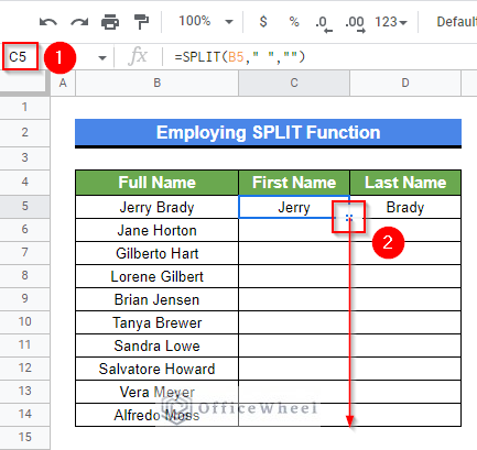
2. Employing SPLIT Function
Instead of using the Split Text to Columns command to paste space or any other delimiter-separated values we can use the SPLIT function to allocate them in adjacent columns. The SPLIT function is an exclusive function in Google Sheets.
Steps:
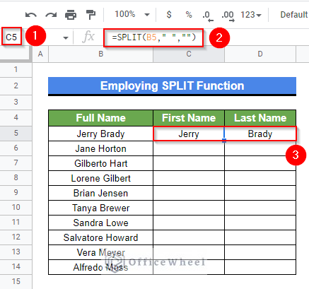
- Firstly, activate Cell C5 by double-clicking on it.
- Then, type in the following formula-
=SPLIT(B5," ","")- Afterward, press the Enter key to get the required output.
- Now, select Cell C5 again and then hover the mouse pointer above the bottom-right corner of the selected cell.
- The Fill Handle icon will be visible at this time.
- Finally, use the Fill Handle icon to copy the formula to other cells of Column C.
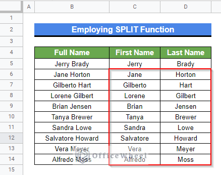
- The final output looks like the following after using the Fill Handle tool.
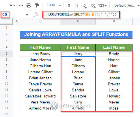
3. Joining ARRAYFORMULA and SPLIT Functions
We can join the ARRAYFORMULA function with the SPLIT function to get the same result as the previous method without using the Fill Handle tool. The SPLIT function is a non-array function. Hence, we require joining the ARRAYFORMULA function with it if we want the SPLIT function to deal with an array.
Steps:
- Activate Cell D5 by selecting it first and then using the function key F2.
- Afterward, insert the following formula-
=ARRAYFORMULA(SPLIT(B5:B14," ",""))- Finally, get the required output by pressing Enter key. And as you can see, we have performed the splitting text operation without using the Fill Handle tool.
Formula Breakdown
- SPLIT(B5:B14,” “,””)
The SPLIT function divides the texts in each cell of range B5:B14 into separate cells of adjacent columns around the space (“ ”) delimiter.
- ARRAYFORMULA(SPLIT(B5:B14,” “,””))
The ARRAYFORMULA function helps the non-array function SPLIT to deal with and display an array.
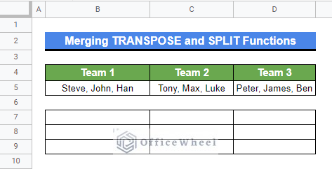
4. Merging TRANSPOSE and SPLIT Functions
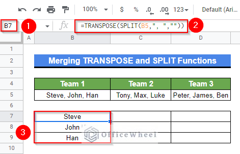
The SPLIT function usually separates values horizontally (adjacent cells of a row). But sometimes, we may require splitting values vertically (adjacent cells of a column) in Google Sheets. We can combine the TRANSPOSE function with the SPLIT function in such scenarios. Let’s have a look at the following dataset. We have the names of the members of the 3 teams. We want to split these names vertically.
Steps:
- First, select Cell B7 and then type in the following formula-
=TRANSPOSE(SPLIT(B5,", ",""))- Next, press the Enter key to get the required result.
Formula Breakdown
- SPLIT(B5,”, “,””)
The SPLIT function first divides the text in Cell B5 into separate cells of adjacent columns around the “, ” delimiter.
- TRANSPOSE(SPLIT(B5,”, “,””))
Later, the TRANSPOSE function converts the rows into columns and columns into rows.
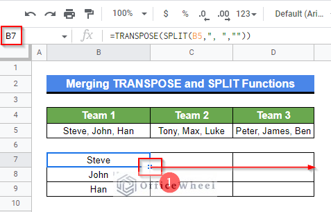
- Now, select Cell B7 again and then hover the mouse pointer above the bottom-right corner of the selected cell.
- The Fill Handle icon will be visible at this time.
- Finally, use the Fill Handle icon to copy the formula to other cells of Row 7.
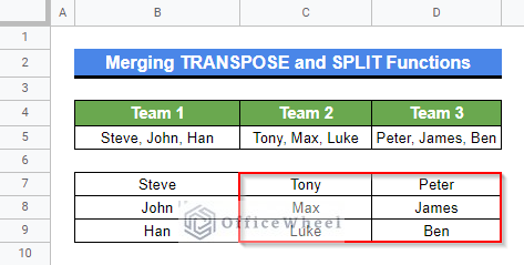
- The final output looks like the following after using the Fill Handle tool.
5. Combining INDEX and SPLIT Functions
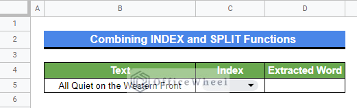
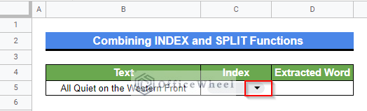
Sometimes, we may require only a specific part of a string. Instead of splitting the entire text, we can simply extract the required part by combining the SPLIT and INDEX functions. We’ll use the following dataset for this example where we’ll extract a specific space-separated word from the data based on an index from a drop-down list.
Steps:
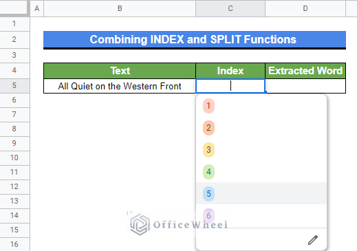
- In the beginning, click on the drop-down icon of the Index column.
- At this time, a list of index options will appear. Select the index you require.
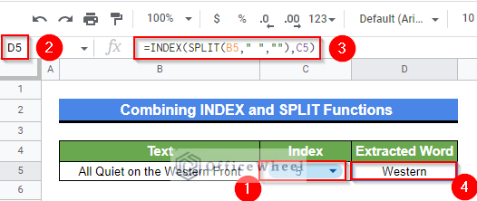
- Now, select Cell D5 and type in the following formula-
=INDEX(SPLIT(B5," ",""),C5)- Finally, press Enter key to get the required result.
Formula Breakdown
- SPLIT(B5,” “,””)
First, the SPLIT function returns a range by dividing each space-separated value into different cells.
- INDEX(SPLIT(B5,” “,””),C5)
Later, the INDEX function returns the content of the cell in the range specified by the SPLIT function based on the offset index provided in Cell C5.
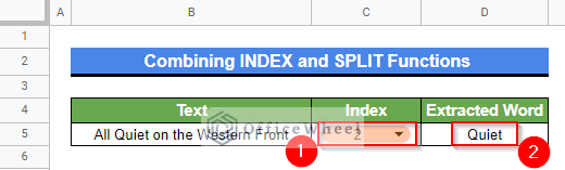
- Now, if we change the index, the extracted word changes automatically.
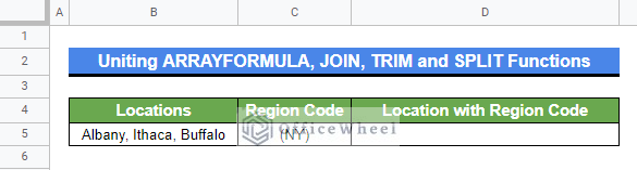
6. Uniting ARRAYFORMULA, JOIN, TRIM, and SPLIT Functions
The SPLIT function can help us to add any specific suffix or prefix to a set of delimiter-separated values when it is united with the ARRAYFORMULA, JOIN and TRIM functions. We’ll demonstrate this example using the following dataset.
Steps:
- First, activate Cell D5 by double-clicking on it.
- Afterward, insert the following formula-
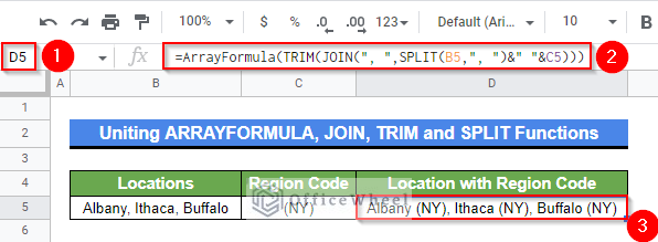
=ARRAYFORMULA(TRIM(JOIN(", ",SPLIT(B5,", ")&" "&C5)))- Lastly, get the required result by pressing the Enter key from your keyboard.
Formula Breakdown
- SPLIT(B5,”, “)
The SPLIT function first divides the texts in Cell B5 into separate cells of adjacent columns around the “, ” delimiter.
- JOIN(“, “,SPLIT(B5,”, “&” “&C5)
Afterward, the JOIN function appends each split value with a space (“ ”) and value stored in Cell C5 around the “, ” delimiter.
- TRIM(JOIN(“, “,SPLIT(B5,”, “)&” “&C5))
Later, the TRIM function removes any leading, trailing, and repeated spaces in the text.
- ARRAYFORMULA(TRIM(JOIN(“, “,SPLIT(B5,”, “)&” “&C5)))
The ARRAYFORMULA function helps to deal with and display an array. Without this, only the first Location-Region value will be shown.
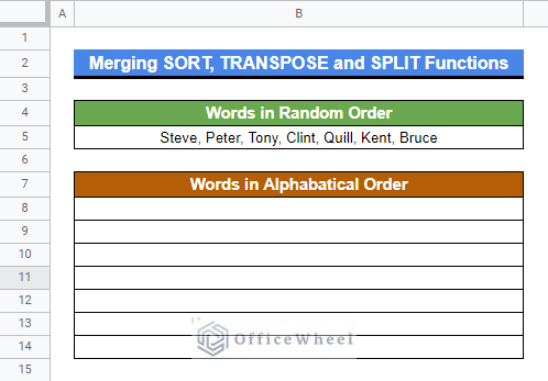
7. Merging SORT, TRANSPOSE, and SPLIT Functions
We can also split a cell vertically to sort the separated values in alphabetical order in Google Sheets. For this, we need to join the SORT, TRANSPOSE, and SPLIT Functions. We’ll use the following dataset to demonstrate this example. We have a list of “, ” delimiter-separated values in a cell that we’ll split and rearrange in alphabetical order.
Steps:
- Select Cell B8 first and insert the following formula-
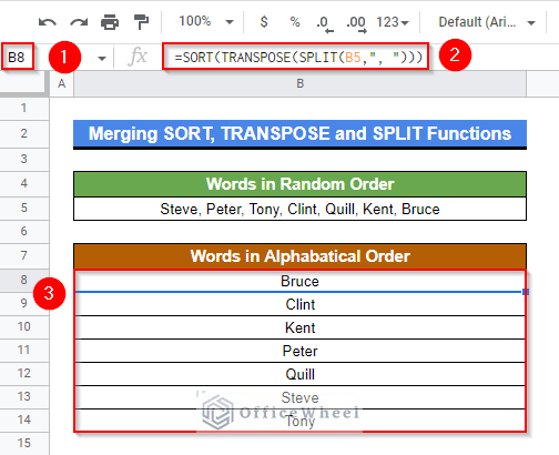
=SORT(TRANSPOSE(SPLIT(B5,", ")))- Now, get the required output by pressing the Enter key.
Formula Breakdown
- SPLIT(B5,”, “)
The SPLIT function first divides the text in Cell B5 into separate cells of adjacent columns around the “, ” delimiter.
- TRANSPOSE(SPLIT(B5,”, “))
Later, the TRANSPOSE function converts the rows into columns and columns into rows. Since the SORT functions require a column to rearrange cells and the SPLIT function returns a row with separated values, we require the TRANSPOSE function.
- SORT(TRANSPOSE(SPLIT(B5,”, “)))
Finally, the SORT function rearranges the rows of a given array or range by the values.
8. Joining QUERY, ARRAYFORMULA, and SPLIT Functions
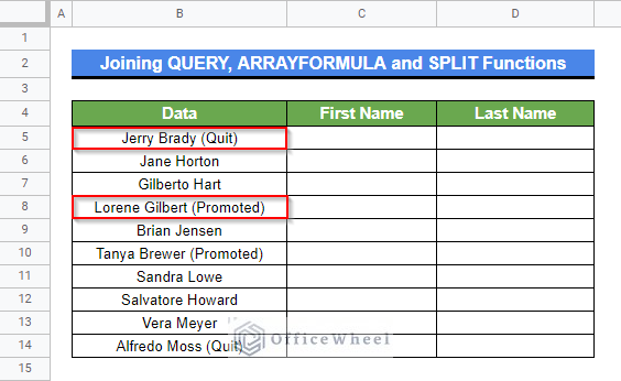
Let’s have a look at the following dataset. The dataset contains several persons’ first and last names and job statuses in a few cells. Now, if we apply the SPLIT function here, we’ll get only first names and last names for a few cells. And in other cells, we’ll also get the job status along with first names and last names. Now, if we only require the first and last names, then we can combine the QUERY function with it to return only first and last names. We’ll also join the ARRAYFORMULA function here to get rid of using the Fill Handle icon. Now, let’s get started.
Steps:
- Firstly, select Cell C5.
- Afterward, type in the following formula-
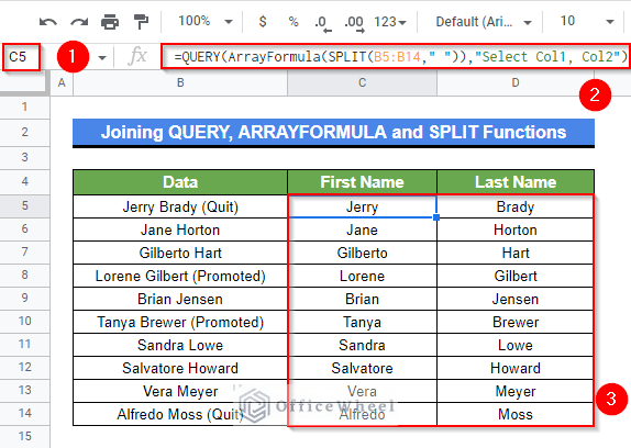
=QUERY(ArrayFormula(SPLIT(B5:B14," ")),"Select Col1, Col2")- Finally, get the required output by pressing the Enter key.
Formula Breakdown
- SPLIT(B5:B14,” “)
First, the SPLIT function divides the texts in each cell of range B5:B14 into separate cells of adjacent columns around the space (“ ”) delimiter.
- ARRAYFORMULA(SPLIT(B5:B14,” “))
Here, the ARRAYFORMULA function helps the non-array function SPLIT to deal with and display an array.
- QUERY(ARRAYFORMULA(SPLIT(B5:B14,” “)),”Select Col1, Col2”)
Finally, the QUERY function runs a Google Visualization API Query Language query across the range returned by the SPLIT function and selects only Column 1 and Column 2 from the range.
9. Combining SPLIT, REGEXREPLACE, and CHAR Functions
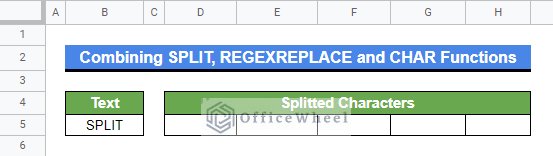
We can combine the SPLIT, REGEXREPLACE, and CHAR functions to separate a word into letters and characters. Splitting up a word into its individual characters may sound quite simple, but it can be a complex approach when automating this process in an application like Google Sheets. We’ll use the following dataset for this example. Now, follow the simple steps below to execute this operation.
Steps:
- To start, select Cell D5.
- Now, type in the following formula-
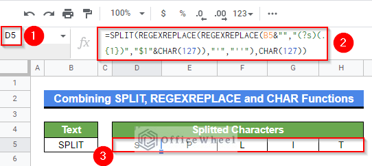
=SPLIT(REGEXREPLACE(REGEXREPLACE(B5&"","(?s)(.{1})","$1"&CHAR(127)),"'","''"),CHAR(127))- Lastly, press Enter key to get the required result.
Formula Breakdown
- CHAR(127)
The CHAR(127) works as a delimiter. In ASCII it is known as the Delete Character. It is virtually invisible and highly likely not to show up in any regular texts or strings.
- REGEXREPLACE(B5&””,”(?s)(.{1})”,”$1″&CHAR(127))
The inner REGEXREPLACE function replaces every character of the word with itself and combines it with a special character CHAR(127). A regular expression flag (?s) is also included that allows the dot (.) to match characters and new lines if there are multiple lines in the reference cell.
- REGEXREPLACE(REGEXREPLACE(B5&””,”(?s)(.{1})”,”$1″&CHAR(127)),”‘”,”””)
The outer REGEXREPLACE function handles any single quotes that might appear in the reference text. It replaces single quotes (‘) with double single quotes (‘’).
- SPLIT(REGEXREPLACE(REGEXREPLACE(B5&””,”(?s)(.{1})”,”$1″&CHAR(127)),”‘”,”””),CHAR(127))
The SPLIT function here uses CHAR(127) as a delimiter to separate the characters of the word here.
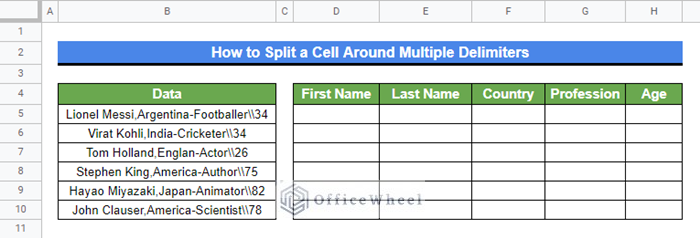
How to Split a Cell Around Multiple Delimiters in Google Sheets
The SPLIT function can only handle one delimiter-separated value. So, how can we deal with multiple delimiter-separated values? We can combine the SPLIT and REGEXREPLACE functions in such scenarios. We’ll use the following dataset for this example. The dataset contains a list of first names, last names, origin countries, professions, and ages for a list of people separated by a space (“ ”), a comma (“,”), a hyphen (“-”) and a double backslash (“\\”) delimiter. Now, let’s perform the splitting operation.
Steps:
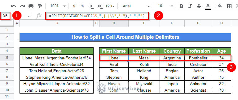
- Firstly, select Cell D5.
- Afterward, insert the following formula-
=SPLIT(REGEXREPLACE(B5,",|-|\\"," ")," ","")- Later, get the required output by pressing the Enter key.
- Finally, Finally, use the Fill Handle icon to copy the formula to other cells of Column D.
Formula Breakdown
- REGEXREPLACE(B5,”,|-|\\”,” “)
The SPLIT function can’t actually divide texts based on multiple delimiters. Hence, the REGEXREPLACE function is used for substituting every other delimiter for a single delimiter. Here, we have substituted every other delimiter with spaces (“ ”).
- SPLIT(REGEXREPLACE(B5,”,|-|\\”,” “),” “,””)
And now, the SPLIT function divides the space-separated values into adjacent cells of a row.
Conclusion
This concludes our article to learn how to split a cell in Google Sheets. I hope the demonstrated examples were ideal for your requirements. Feel free to leave your thoughts on the article in the comment box. Visit our website OfficeWheel.com for more helpful articles.