COUNTIF Multiple Criteria in Google Sheets (3 Ways)

A veteran in Excel will tell you how powerful the COUNTIF function and all its iterations are. The same importance is carried over to Google Sheets.

In this article, we will be looking at how we can count with multiple criteria with COUNTIF, its close iterations, and a couple of alternatives, in Google Sheets.

Let’s get started.

COUNTIF for Multiple Criteria in Google Sheets- AND Logic

1. Using COUNTIFS for Multiple Criteria

The simplest way to count for criteria in Google Sheets is to utilize the COUNTIFS function. This function was literally created for such situations.

The COUNTIFS function syntax:

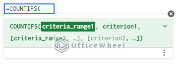
• criteria_range1: The range of cells that we will check
• criterion1: The value that we will check the range with
• [criteria_range2, criterion2]: Optional. The second section of the range and criterion.

More criteria can be added accordingly.

To showoff this function, we have a simple dataset on which we can perform counts based on multiple conditions:

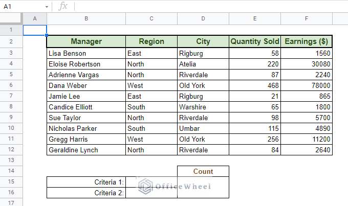
For our first count, our conditions will be: More than 100 units sold in the northern region.

1. Quantity Sold: >100
2. Region: North

Let’s put these conditions into action.

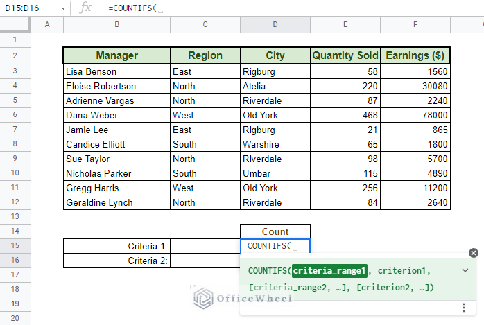
Step 1: Select the cell where you want your count to be and type =COUNTIFS(

Step 2: Add the two conditions with their respective ranges:

Criteria 1: E3:E12,”>”&100

Criteria 2: C3:C12,”North”

Our final formula:

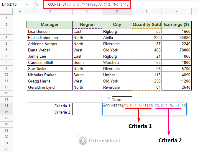
Step 3: Close parentheses and press ENTER

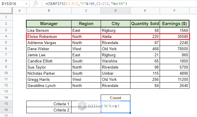
We have successfully counted the number of records in our dataset that satisfies multiple criteria!

Note that the greater than symbol (>) is within quotation marks (“”) as it is seen as a text value, and it is concatenated with the numerical value, 100, with an ampersand (&).

We can avoid this by directly using cell references for our conditions:

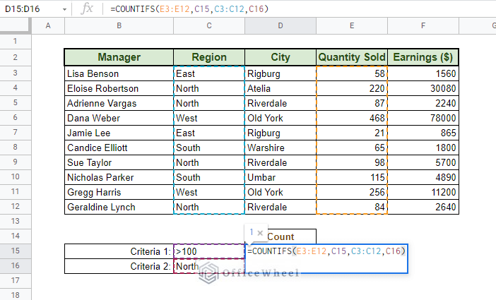
From this point forward, we will be utilizing cell references for our criteria.

2. Using COUNTUNIQUEIFS Function

The COUNTUNIQUEIFS function is a great spin on the base COUNTIFS function. It fundamentally works the same way, but it only considers unique records in the range designated by the user.

COUNTUNIQUEIFS Syntax:

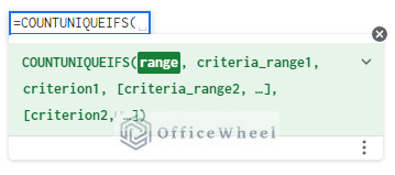
• count_unique_range: The range reference from which the unique values will be counted.
• criteria_range1: The range of cells that we will check
• criterion1: The value that we will check the range with
• [criteria_range2, criterion2]: Optional. The second section is of range and criterion.

The count_unique_range virtually acts as a criterion on its own.

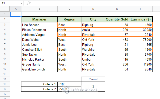
For our test, we will be counting all the unique regions that have less than 100 products sold and have an earning lower than $5000.

• Unique range: C3:C12
• Criteria 1: E3:E12,C15
• Criteria 2: F3:F12,C16

Final Formula:

According to COUNTIFS criteria, the following records satisfies the conditions:

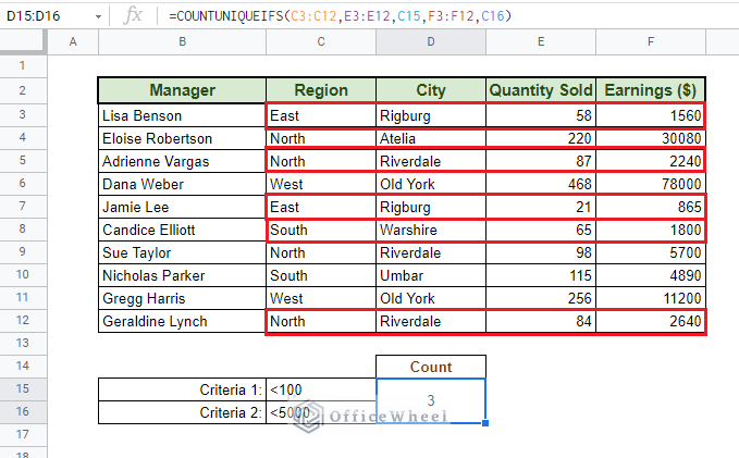
But COUNTUNIQUEIFS will take these 3 unique values:

COUNTIF for Multiple Criteria in Google Sheets – OR Logic

By default, the COUNTIF function only works with one range and one criterion. However, you can add or subtract or combine other functions with it to give an overall count. But this is only for a single type of data or column of data.

So, it is highly unlikely you will need to make it so complex when you have a function like COUNTIFS available. But we are going to see how we can achieve this anyways.

1. Adding Counts: COUNTIF + COUNTIF

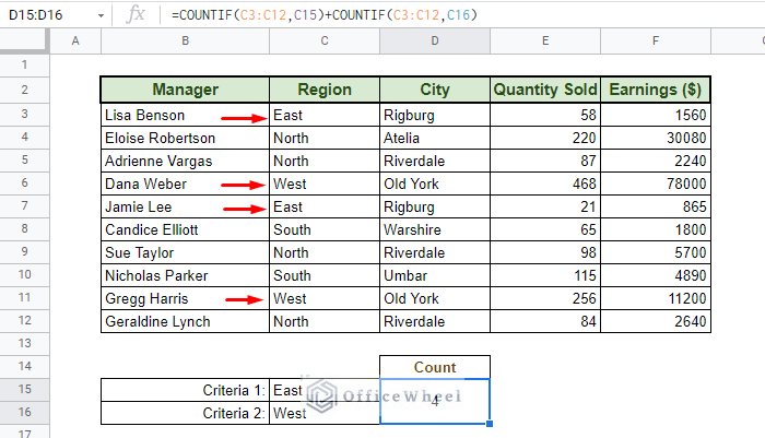
For our example, we will be counting the number of records of regions East and West.

The formula is simple, we will add two instances of the COUNTIF function:

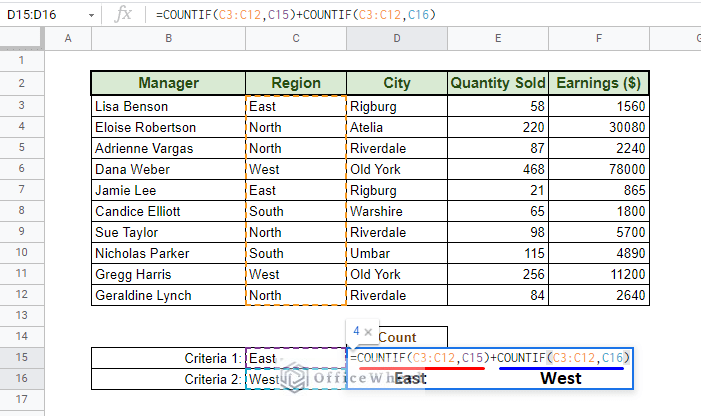
We have two East records and two West records:

2. Subtracting Counts: COUNTIF – COUNTIF

Now, we are going to find the number of records between a range of numbers, namely, the records that have a Products Sold value between 100 and 300.

Since we cannot put both number conditions in a single COUNTIF, we will be subtracting the count of one range from the other:

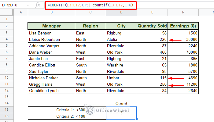
Records under 300: COUNTIF(E3:E12,C15) = 9

Records under 100: COUNTIF(E3:E12,C16) = 6

9 – 6 = 3

Easy.

3. Single Column, Multiple Criteria with COUNTIFS

If we want to use multiple criteria in the same column with COUNTIFS, we have to make use of the OR logic and array values. Array values are denoted to be enclosed in curly braces {}.

Our idea is simple for our example. Like we have seen previously, we will be summing all the instances that have a region value of East and West.

A point to note before we dive in, Google Sheets works with arrays differently compared to Excel. For Sheets, we have to use the function ARRAYFORMULA when we are working with a formula that has array values.

That said, our formula this time will be:

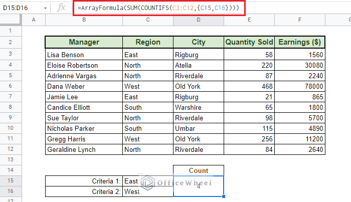
You can replace cell references C15 and C16 with “East” and “West” respectively.

Alternatives

1. QUERY

QUERY is a pretty powerful function in Google Sheets. If you can work with it, you can replicate virtually any other formula, even COUNTIFS. This makes QUERY the perfect alternative function to COUNTIF for multiple criteria in Google Sheets.

To show it off, let’s bring down the COUNTIFS formula that we have used before:

Its equivalent QUERY formula will be:

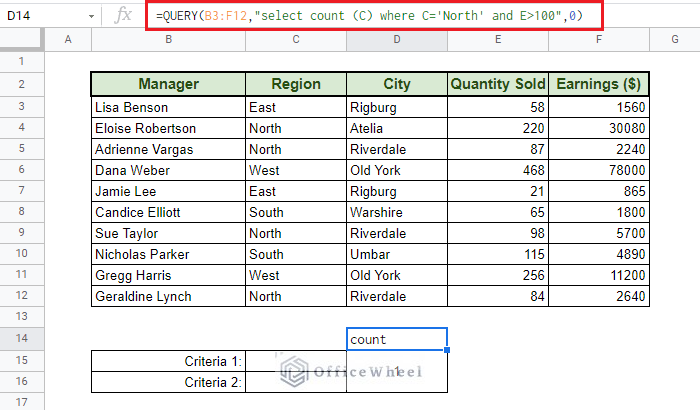
Formula Breakdown:

• B3:F12: Our data range
• select count (C): We are counting for the data in column C
• where C=’North’ and E>100: Our two criteria
• 0: No headers were selected

Note: “count” is an automatic header of the query.

2. SUMPRODUCT

The other alternative we are going to be discussing today is the SUMPRODUCT function.

We will again apply the COUNTIFS equivalent formula (=COUNTIFS(E3:E12,">"&100,C3:C12,"North") in a SUMPRODUCT version:

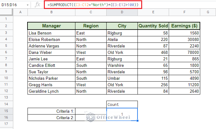
Final Words

We hope that we were able to make to grasp the fundamentals and the different processes through which you can COUNTIF for multiple criteria in Google Sheets. Hopefully, you can now use them with ease in your spreadsheets.

Feel free to leave a comment with any queries or advice you might have.

Related Articles for Reading

• Count Duplicates In Google Sheets (3 Ways)
• COUNTIF From Another Sheet in Google Sheets
• COUNTIF Across Multiple Sheets in Google Sheets