How to Use the Find Function in Google Sheets (An Easy Guide)

The FIND function comes in handy when you want to search for a keyword with a piece of text or string. And with enough understanding and creativity, we can take it a step further.

So today, in this simple tutorial, we will show you how to use the FIND function in Google Sheets and what else we can do with it.

Let’s get started.

What is the FIND Function in Google Sheets?

Let’s say that you want to find the exact position of a letter or a keyword from a text or string in Google Sheets.

Is there a function in Google Sheets that does that?

That’d be the FIND function.

The FIND function returns the exact position of a letter or keyword found in a given string.

FIND also has the advantage of also allowing the user to optionally set the starting point of the search in the string.

Let’s now look at the breakdown and a basic example of the Find function of Google Sheets.

The FIND Function Breakdown

The syntax of the FIND function:

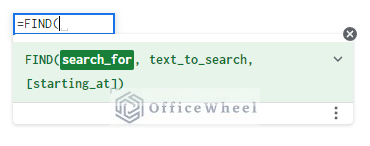
Breakdown:

• search_for: The letter/keyword/string that you are looking for. Must be enclosed in quotation (“”) or it can be presented as a cell reference.
• text_to_search: The text or string on which the search occurs for the first occurrence of search_for. Must be enclosed in quotation (“”) or it can be presented as a cell reference.
• [starting_at]: This field is optional. The starting position of the search in the text or string. Only takes integer values.

Basic Example

Let’s look at a couple of basic uses of the FIND function.

The first is:

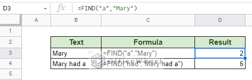
It looks for the first occurrence of “a” in the text. We have found it in position 2.

The second is:

It looks for the first occurrence of “had”. This string has more characters, but the function was able to find it. The keyword starts from position 6. Note that the FIND function counts spaces as a position.

Read More: How to Search in All Sheets in Google Sheets (An Easy Guide)

Points to Note about the FIND Function

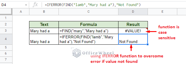
1. The FIND function is case-sensitive. You must be careful when you are searching for upper- or lower-case letters or keywords.
2. The starting position (starting_at field) value must be an integer greater than or equal to 1. Since the first character of the text is considered to be 1.
3. Like many other text functions, FIND can utilize wildcards to customize search. The three wildcards are the asterisk (*), question mark (?), and tilde (~).
4. When a value is not found, the find function will return an error (#VALUE). So it is best to encapsulate the function inside an error handling function like IFERROR.

Read More: Find and Replace with Wildcard in Google Sheets

How to use the FIND Function in Google Sheets

Practical Example: Find a Substring from a Text in Google Sheets

Commonly, we utilize the FIND function to find the presence of a substring in a line or paragraph of text. Let’s go through this process step-by-step.

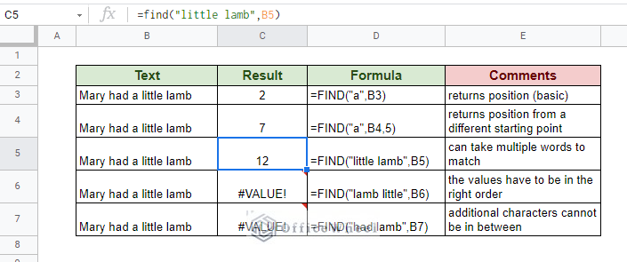
Step 1: Open the FIND function at the desired location by typing =FIND(. Google Sheets should automatically present you with a suggestion.

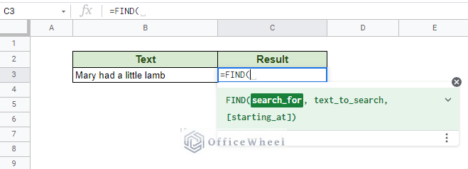
Step 2: Type in the letter or keyword you are looking for in quotation (“”). We have chosen the word “little”.

Step 3: Now, instead of writing out the whole sentence, we have opted to use a cell reference to our text. Our text is in cell B3.

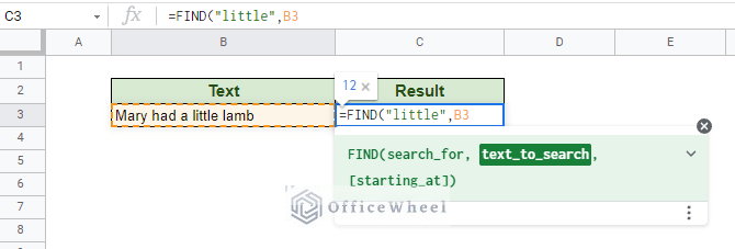
Step 4: Close parentheses and press ENTER.

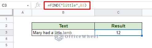
The exact match was found at position 12.

But this result may not be of any practical use unless you only want the position.

What we want is a meaningful message stating whether a match was found or not.

Read More: How to Compare Text in Google Sheets (3 Easy Ways)

Applying an IF Statement with FIND Function for a Meaningful Output

To produce a meaningful output, we can simply apply an IF condition. This IF function will take advantage of ISERROR to give outputs for results found and not found (remember that no match results in an error).

Since ISERROR returns TRUE if an error (no match) is found, our formula will be:

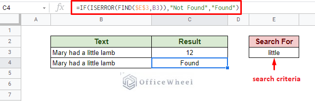
Note: We have used absolute cell reference ($E$3) to always point to the single search criteria.

This is a huge advantage over something like the MATCH function which cannot search for keywords within a string.

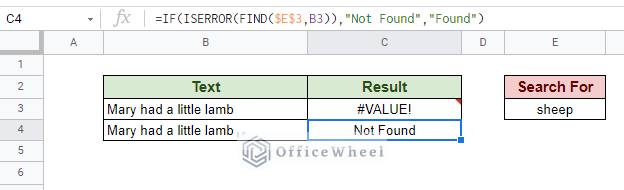
When the formula cannot find the keyword:

To round off the general use of the FIND function, here are some iterative examples of how we can use it:

Read More: How to Search in Google Spreadsheet (5 Easy Ways)

Similar Readings

• How to Count Unique in Google Sheets (3 Easy Ways)
• Find Uncertainty of Slope in Google Sheets (3 Quick Steps)
• How to Find Correlation Coefficient in Google Sheets
• Replace Space with Dash in Google Sheets (2 Ways)
• How to Apply a Custom Sort in Google Sheets

Search for Text Over a Range Using FIND Function

It is 100% possible that you may only have a single keyword to search for in a range of cells or a column. In such cases, writing a FIND formula for each row may be impractical.

The FIND function thankfully allows us to input a range in the text_to_search field so that we can search for our keyword over the entire column.

However, on its own, FIND will only return the first result. Here is where ARRAYFORMULA comes in handy.

Our FIND formula to search over a range is:

Enclose it in ARRAYFORMULA to present all the results. You can press CTRL+SHIFT+ENTER instead of just ENTER to apply ARRAYFORMAL around the current formula:

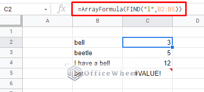
The formula is quick, can be used for any column range and you only have to use it once.

Read More: How to Use ARRAYFORMULA in Google Sheets (6 Examples)

FIND vs SEARCH

Any long-time user of Google Sheets will be aware of another similar function to FIND, the SEARCH function.

It has been the topic of many discussions about any differences between them. This query generally stems from the virtually identical parameters that the FIND and SEARCH functions have.

The SEARCH function syntax:

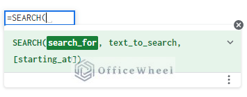
There is but only one key difference in functionality that set them apart:

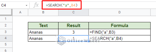
The FIND function is not case sensitive whereas the SEARCH function is.

Final Words

That concludes our very simple guide on how to use the FIND function in Google Sheets. The positional value that the function returns can be utilized on its own, or it can be combined with others to give a more customized and meaningful outcome.

Feel free to leave any queries or advice you might have for us in the comments section below. Or have a look at the other search-related articles we have here.

Related Articles for Reading

• How to Use ARRAYFORMULA with IF Function in Google Sheets
• Find and Replace in Google Sheets (3 Ways)
• How to Find and Delete in Google Sheets (An Easy Guide)
• Find All Cells With Value in Google Sheets (An Easy Guide)
• How to Sum Using ARRAYFORMULA in Google Sheets
• Find Value in a Range in Google Sheets (3 Easy Ways)
• How to Use Find and Replace in Column in Google Sheets