How to Substitute Multiple Values in Google Sheets (An Easy Guide)

In this simple tutorial, we will look at how we can substitute multiple values in Google Sheets.

Unsurprisingly, our primary method revolves around the SUBSTITUTE function. However, we will have a look at a great alternative later.

Let’s get started.

How to Substitute Multiple Values in Google Sheets

To show the methods, we will use the following worksheet where we have a bunch of IDs along with their product names:

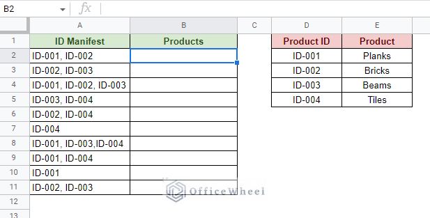
Our objective here is to substitute or replace the IDs with their respective names. And we will do this using the SUBSTITUTE function.

The SUBSTITUTE function syntax:

As a simple example, let’s substitute ID-001 with Planks. You can skip ahead to the next section for multi-substitutions.

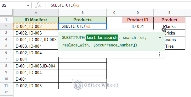
Step 1: Open the SUBSTITUTE function and select the source data reference.

Step 2: Input the old text to replace. Then input the substitute text after a comma. Make sure both values are inside quotations (“”).

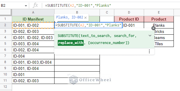
Google Sheets will provide a preview of the results.

Step 3: Close parentheses and press ENTER to see the result. And use the fill handle to apply the formula to the rest of the column.

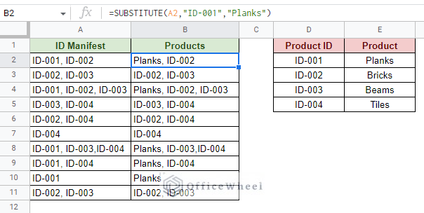
As you may have noticed from this example, the SUBSTITUTE function cannot take multiple values to replace. So, we have to get a little creative to substitute multiple values with the SUBSTITUTE function in Google Sheets.

Read More: How to Use Find and Replace in Column in Google Sheets

Using the SUBSTITUTE Function to Replace Multiple Values

While the SUBSTITUTE function cannot replace multiple values, we can use multiple SUBSTITUTE functions in a single formula to do so. We do this by nesting multiple SUBSTITUTE functions according to the number of values we want to replace.

Therefore, to substitute ID-001 and ID-002 with Planks and Bricks respectively, the formula syntax will be:

Making the final formula for substituting the two values:

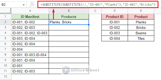
Then, use the fill handle to apply the formula to the rest of the column.

Finally, the formula for all four IDs with their respective product names is:

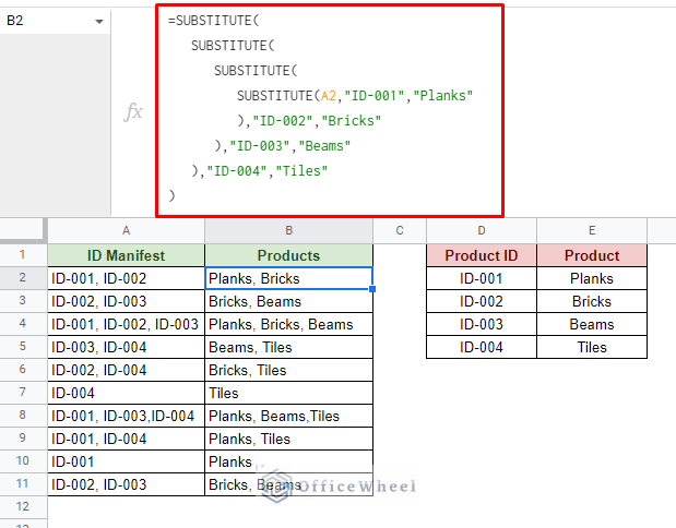
Read More: Easy Guide to Replace Formula with Value in Google Sheets

Using Cell Reference to Substitute Multiple Values in Google Sheets

Cell references are a great way to input values easily and quickly in formulas, especially when you have so many that we have seen with SUBSTITUTE with multiple values.

We already have the reference table for the cell references in the worksheet:

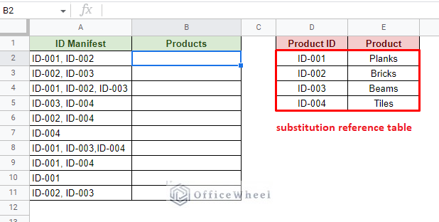
All we have to do is reference the Product ID values as old_text and Product names as the new_text respectively in the formula:

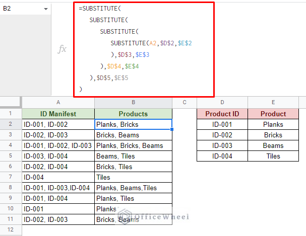
A crucial point to note here is that every cell reference beyond the source data (cell A2 and other values in the ID Manifest column) is locked with absolutes ($). This is to prevent the cell references from moving as we use the fill handle to apply the formula down the column.

Note: You can easily lock cells by selecting the cell reference and pressing the F4 key on the keyboard.

Similar Readings

• How to Search in Google Spreadsheet (5 Easy Ways)
• Find Uncertainty of Slope in Google Sheets (3 Quick Steps)
• How to Find Correlation Coefficient in Google Sheets
• Replace Space with Dash in Google Sheets (2 Ways)
• How to Find Trash in Google Sheets (with Quick Steps)

Extra: Use ARRAYFORMULA to Only Apply the Formula in a Single Cell

The idea behind using cell references to import values was to make the formula easier to use. What if we said we can make it even more dynamic?

We can do this with the application of the ARRAYFORMULA function to allow the SUBSTITUTE function to take a range of values. Specifically, the source data that is in the ID Manifest column.

Step 1: After inputting the SUBSTITUTE formula, press CTRL+SHIFT+ENTER to apply the ARRAYFORMULA around it.

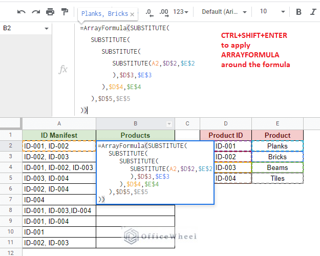
Note: You can also manually input the ARRAYFORMULA around the formula.

Step 2: Update the source data range of the SUBSTITUTE function, A2 to A2:A11 or A2:A.

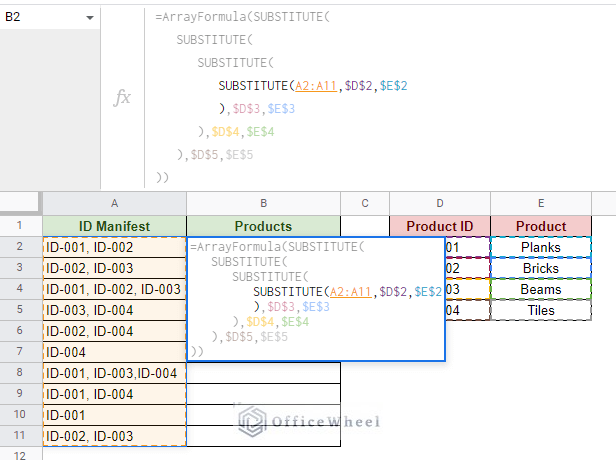
Step 3: Press ENTER to apply.

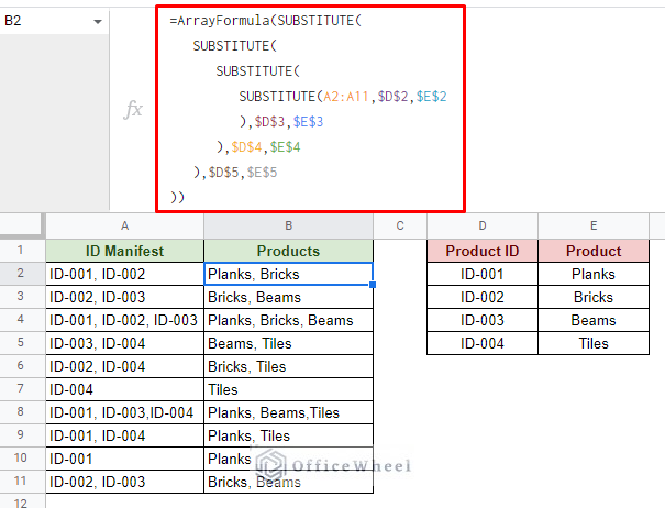
Advantages of using ARRAYFORMULA:

1. The final formula only occupies one cell in the column.
2. Calculation and processing of the function are much faster. Makes the worksheet more efficient.
3. Locking cell references are not necessary (even though our image shows it) since the fill handle is not used to apply the formula down the column.

Important Note: You can also use the REGEXREPLACE function in place of SUBSTITUTE if you are looking for more freedom to apply text conditions with regular expressions. The syntax is the same in this scenario.

Read More: Use REGEXREPLACE to Replace Multiple Values in Google Sheets (An Easy Guide)

Alternative: Using VLOOKUP to Substitute Multiple Values in Google Sheets

If you have been using spreadsheet applications for a while, then you’ll be familiar with the VLOOKUP function.

The function essentially searches for a user-defined value over a known range. In this section, we will take advantage of this feature to search and substitute values in Google Sheets.

The other functions we will use alongside this formula are:

• SPLIT: To separate values by commas (,) from the source data.
• TRIM: To remove blank spaces.
• TRANSPOSE: To help list the values found.
• VLOOKUP: To search for the given values.
• IFNA: To handle the #N/A error when VLOOKUP does not find any matches.
• TEXTJOIN: To bring all the values together separated by a comma and a space.
• ARRAYFORMULA: To accommodate a range of cells given in the curly braces {} (given as an array value).

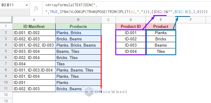
The final formula:

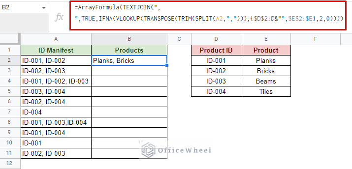
Use the fill handle to apply the formula to the rest of the column.

Advantages:

1. The formula is completely dynamic when it comes to searching and replacing values. You can notice that from the range of the old text (D2:D) and new text (E2:E).
2. You can simply copy-paste the formula to use. So, you only have to change the cell references.

Disadvantages:

1. Unlike what we’ve seen with the previous ARRAYFORMULA example, this function requires you to use the fill handle and drag it down the column to apply.
2. The formula will substitute values that don’t match with a blank space. E.g., If there was an ID-005 in the ID Manifest column and not in the reference range (columns D and E) the value will be output as a blank.

Final Words

That concludes our simple guide on how to substitute multiple values in Google Sheets. While our function of choice has been SUBSTITUTE unsurprisingly, there are other approaches that we can take, like REGEXREPLACE or VLOOKUP compound formulas.

Feel free to leave any queries or advice you may have for us in the comments section below.

Related Articles for Reading

• How to Remove Special Characters in Google Sheets (3 Easy Ways)
• Find and Replace in Google Sheets (3 Ways)
• How to Find Hidden Rows in Google Sheets (2 Simple Ways)
• Find Value in a Range in Google Sheets (3 Easy Ways)
• How to Find Median in Google Sheets (2 Easy Ways)
• Find and Replace with Wildcard in Google Sheets
• How to Find Edit History in Google Sheets (4 Simple Ways)
• Find Frequency in Google Sheets (2 Easy Methods)