Google Sheets UNIQUE function helps to quickly identify the unique values in the spreadsheet. When working with a larger dataset, this function comes in quite handy. The best characteristic of the UNIQUE function is that it discards identical values. This article will demonstrate the various applications of the UNIQUE function.
A Sample of Practice Spreadsheet
You can copy the spreadsheet that we’ve used to prepare this article.
What Is the UNIQUE Function in Google Sheets?
In general, the UNIQUE function can extract a list of distinct values by removing duplicates, i.e. unique values, and returns data in rows from the specified source range. The values are returned in the order they first appear.
Syntax
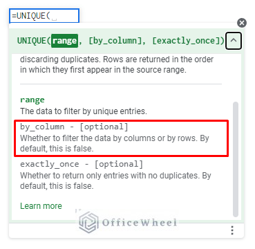
The UNIQUE function has the following syntax.

Argument
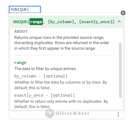
The arguments of the UNIQUE function are as follows:
| Argument | Requirement | Function |
|---|---|---|
| range | Required | The range to be filtered by unique entries |
| by_column | Optional | It filters data by columns or rows. By default, it is False. |
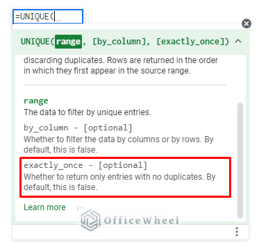
| exactly_once | Optional | Return values that have no duplicates. By default, it is False. |
Output
The formula =UNIQUE(B6:B15) will return distinct values in the cell range B6:B15.
5 Useful Applications of UNIQUE Function in Google Sheets
The UNIQUE function in Google Sheets may be used in a variety of ways, and we will do our best to demonstrate them all in this article.
1. General Use of UNIQUE Function
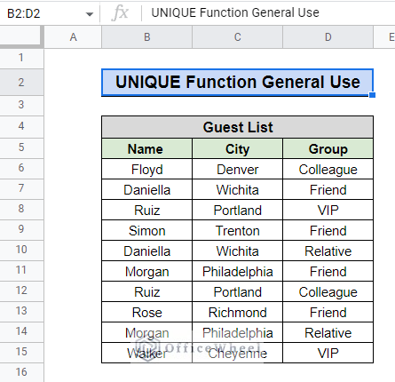
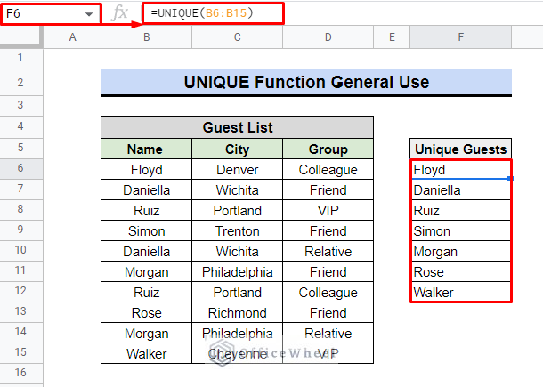
First of all, we’ll demonstrate how to use the UNIQUE function in its most fundamental form. Assume we have a guest list with names, their city of residence, and the group to which they belong. We will now search the guest list for unique names. Because some guests belong to more than one group.
Steps:
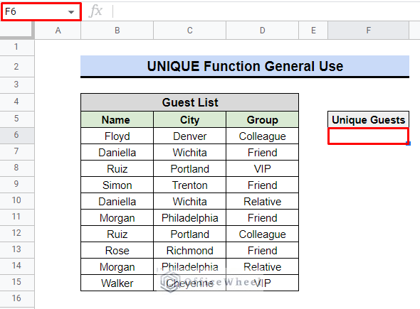
- In cell F5, let us create a new column header labeled Unique Guests.
- After that, we’ll choose cell F6 to place the formula in.
- We will use the following Formula:
=UNIQUE(B6:B15)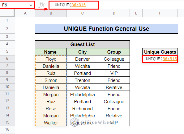
- To activate the function, press ENTER.
The names are listed in a box directly beneath the Unique Guest Header. There are no longer any repeated values or names.
In the following subsection, we’ll examine each argument of the UNIQUE function.
I. Setting by_column Condition
In general, this argument focused on whether to filter data by rows or columns. As this function primarily focuses on rows for distinct values, it is set to FALSE by default.
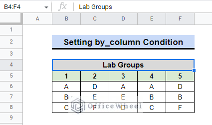
However, we shall use a simple example to illustrate the condition if we want to filter data by column. Assume there are 5 lab groups of 6 students. We need to identify and eliminate duplication.
Steps:
- To begin, we’ll make a Unique Group header in cell B11.
- Select cell B12, which is located below the header.
- We shall apply the following formula:
=UNIQUE(B6:F8,TRUE)- We’ll press ENTER to finish things off.
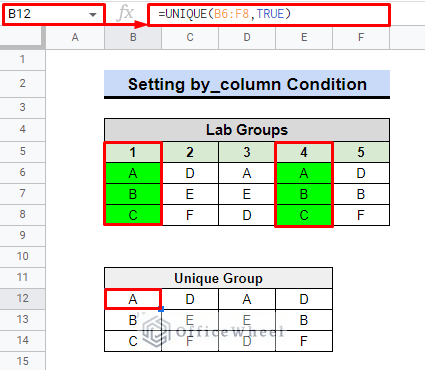
The duplicate columns, which were later removed by the UNIQUE function just because we utilized the by_column argument, are highlighted in the image above.
Read More: How to Get Unique Values Without Blanks in Google Sheets
II. Setting exactly_once Condition
We may retrieve the data that don’t have any repeated values by using the following feature of the UNIQUE function. The default value of this argument is FALSE since it typically displays both the common value without duplication and values that have only appeared once.
Values that have only ever appeared once will emerge. For this scenario, we’ll once more use the guest database as an example. Check the steps below.
Steps:
- Firstly, we will select cell F6.
- Secondly, We will use the following formula:
=UNIQUE(B6:B15,FALSE,TRUE)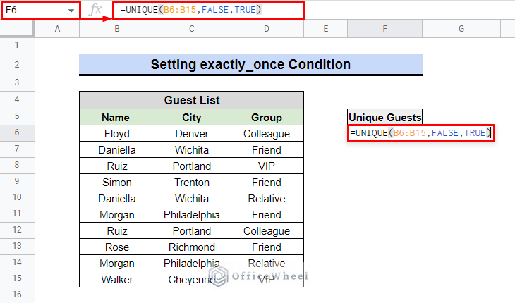
- Finally, We will press ENTER to conclude.
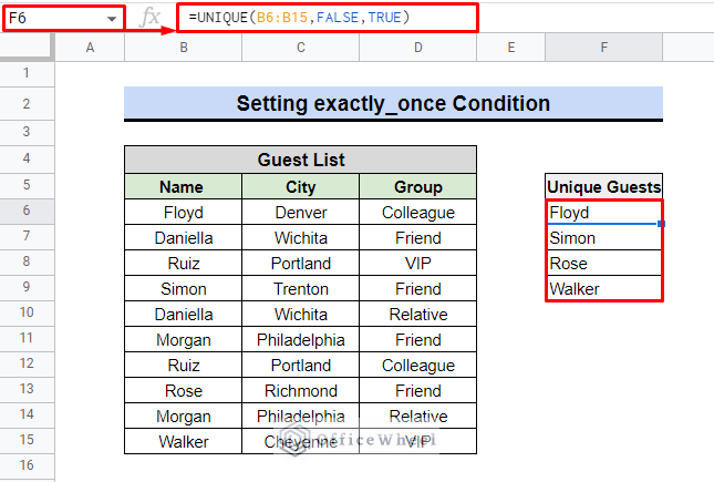
There are no repeated entries for these four guests because they share only one kind of relationship. As a result, they were put in the column below for Unique Guests.
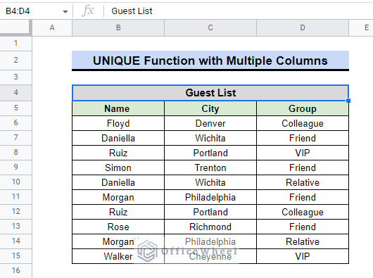
2. UNIQUE Function with Multiple Columns
We can also extract unique values from multiple columns. Assume we’re going to bring up both the unique guests and their place of residence or the name of the city at the same time.
Steps:
- We’ll create two new header columns. The first is Unique Guests, and the second is Unique City in cells F5 and G5.
- The next step is to enter the following formula by clicking cell F6.
- To find the distinct values, we shall apply the following Formula:
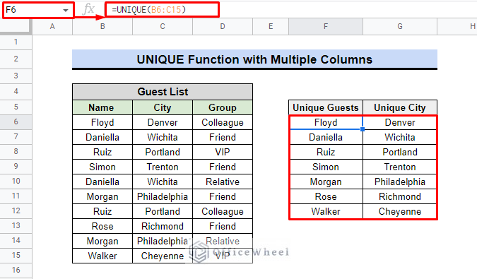
=UNIQUE(B6:C15)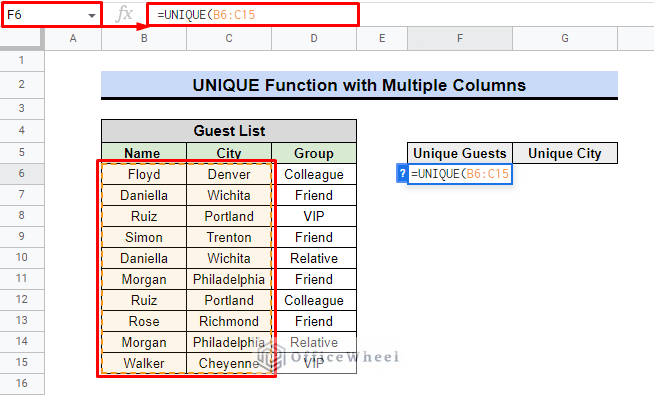
- To view the outcome, press ENTER.
In the F and G columns, respectively, the function listed the names of the guests and the cities.
Read More: How to Count Unique Values in Multiple Columns in Google Sheets
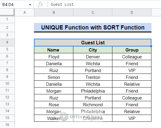
3. Use of UNIQUE and SORT Functions
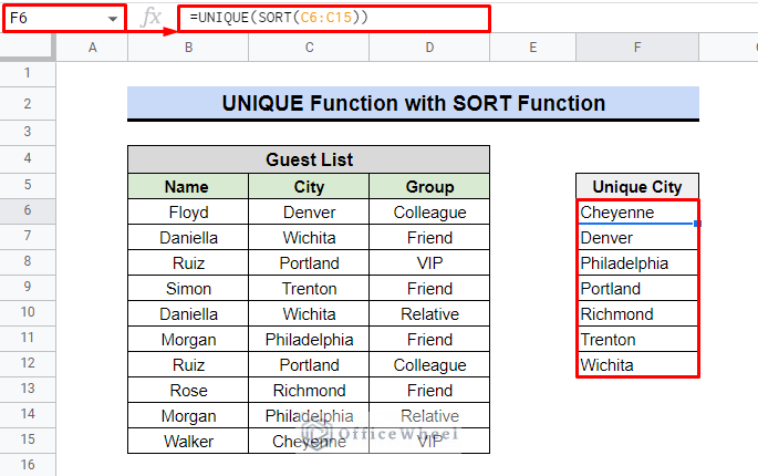
Because the SORT function assists in sorting the data in descending order, using it in combination with a UNIQUE function produces better-structured results. Consider that we are bringing out the city names by removing duplicates, but this time they are in alphabetical order.
Steps:
- In cell F5, we must once more open a new column header called “Unique City“.
- We’ll use the following formula in cell F6 just below.
Formula:
=UNIQUE(SORT(C5:C15))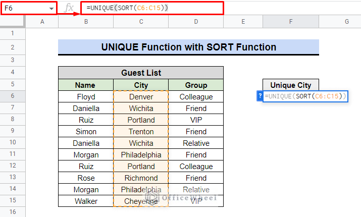
- Lastly, press ENTER.
If we look closely, we can see that the city names are listed from A to Z in alphabetical order.
Similar Readings
- How to Apply QUERY for Unique Rows in Google Sheets (4 Ways)
- Highlight Unique Values in Google Sheets (9 Useful Ways)
- How to Remove Unique Values in Google Sheets (2 Suitable Ways)
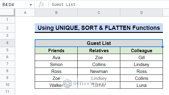
4. Advanced Use with SORT & FLATTEN Functions
The UNIQUE function has a broader application when the SORT and FLATTEN functions are added. To make the point apparent, we’ll provide an example.
Assume we have a list of three different guest groups. Some individuals, however, belong to multiple groups because they share multiple relationships. We will now eliminate duplicates and list each guest in a precise order.
Steps:
- Once more, we’ll add a new header labeled “Unique Guests” to cell F5.
- Then, in cell F6, we’ll use the following
- We will use the following combination as Formula:
=UNIQUE(SORT(FLATTEN(B6:D10)))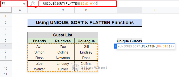
- In order to finish the formula, press ENTER.
We will find that the formula lists each guest in descending order.
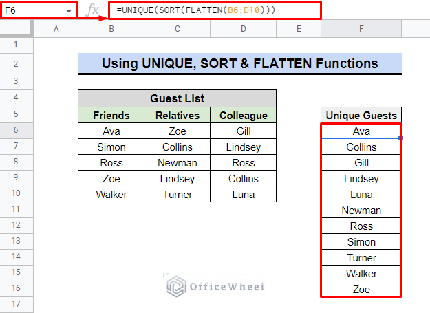
Formula Breakdown:
- FLATTEN function will combine all of the values in cells B6 to D10.
- The SORT function will sort the values returned by the FLATTEN function.
- After the values are returned by the SORT function, The UNIQUE function will delete duplicate values.
5. UNIQUE Function with Horizontal Data
Up to this point, we have solely used vertical data. The UNIQUE function typically operates row-wise. It may work with either column data or horizontal data, albeit, with the aid of the TRANSPOSE function. To better explain its application, let’s go through the scenario below.
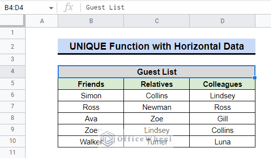
Consider using the UNIQUE function in rows to eliminate repetitions. We will work with all the columns of row 7 in this situation.
Steps:
- In column F, cell F5, insert a new heading as Unique Guests.
- We’ll apply the following formula in cell F6 after that.
=UNIQUE(SORT(TRANSPOSE(B7:D7)))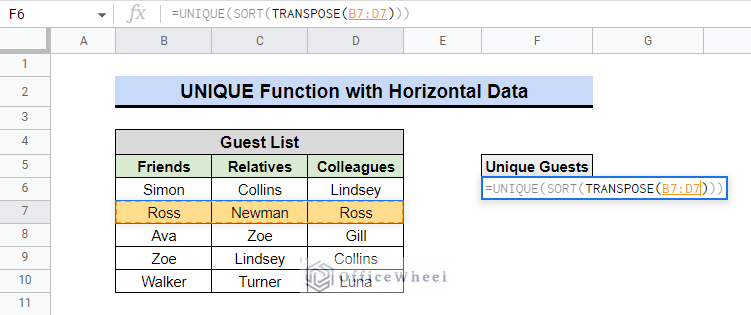
- To see the outcome, press ENTER.
Row 7 clearly has two Ross. Because of the formula, one of them is discarded, and only unique values are returned.
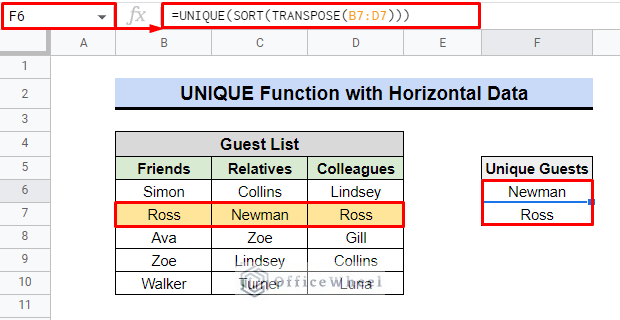
Formula Breakdown:
- In the cell range B7:D7, the TRANSPOSE function reversed the column values in the row.
- When the TRANSPOSE function returned values, the SORT function sorted them.
- The UNIQUE function eliminated the duplicate values returned from the previous operation.
Conclusion
There are a variety of other situations in which you might use the UNIQUE function. These are all, however, only the actual uses of the Google Sheets UNIQUE function. Please leave a comment if you have any questions. For additional information, visit OfficeWheel.