Today, we will look at a couple of ways with which we can find cell references in Google Sheets, focusing on the ones that can be found in formulas.
Let’s get started.
2 Ways to Find Cell Reference in Google Sheets
In a worksheet, the only place you can find cell references to other cells is inside a formula. That is why it can get quite difficult to correct any cell misreferences in a worksheet.
To find these cell references, we can take two approaches, depending on where and what we are looking for:
- Find and Replace
- Using the CELL function
1. Using the Find and Replace Option of Google Sheets
Find and Replace is a built-in search option of Google Sheets. You might be thinking it to the traditional CTRL+F search bar, but it is much more than that.
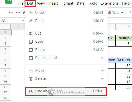
To access it, simply use the keyboard shortcut CTRL+H or navigate to the option from the Edit tab.
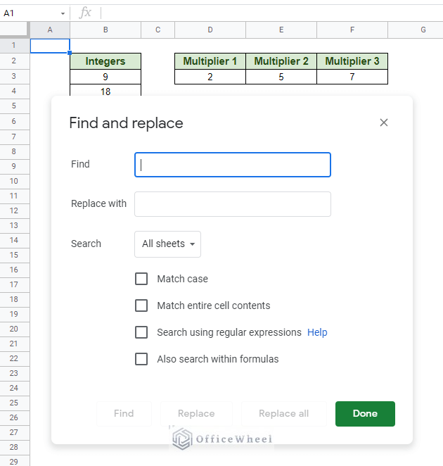
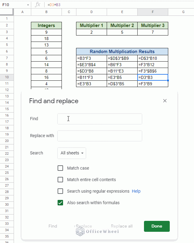
The Find and Replace Window
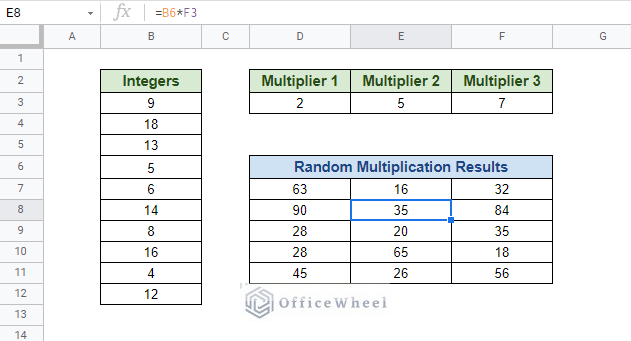
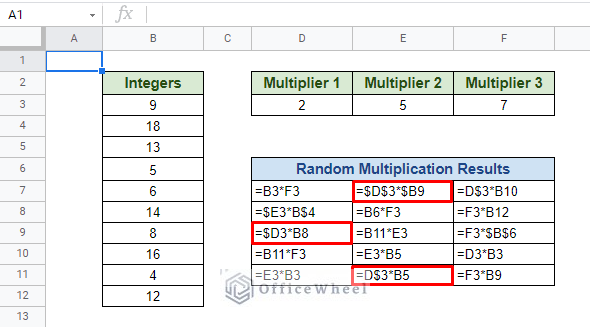
To show how we can find cell references with Find and Replace, we have the following worksheet of Integers, Multipliers, and some randomized results of the two in a table.
Obviously, the Randomized Multiplication Results contain cell reference formulas on which we are going to perform the search on.
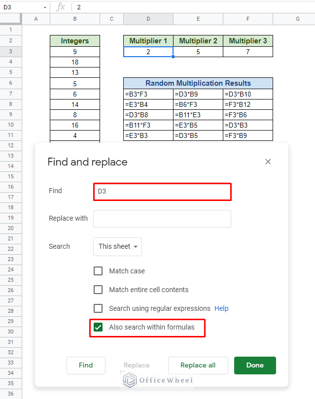
So, open the Find and Replace window to search for, let’s say D3, which is the cell reference of the multiplier 2.
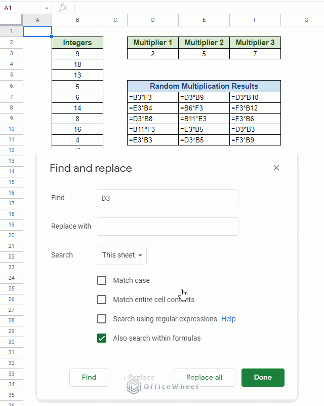
It is very important to check the Also search within formulas option. This will reveal all the cells that contain formulas. Click Find to begin the search.
With each click of Find, the application cycles through every instance of the search criteria through the worksheet.
The Disadvantage of Find and Replace
We may find ourselves with formulas that have locked cell references in them. The Find function searches cannot recognize these locked cells due to the presence of absolutes ($) ($D$3, D$3, or $D3), unless these absolutes are defined in the Find criteria.
That is somewhat impractical as we have three different ways to lock cells in Google Sheets and searching for each type individually will cost more than just time.
Read More: Variable Cell Reference in Google Sheets (3 Examples)
Similar Readings
- [Fixed!] INDEX MATCH Is Not Working in Google Sheets (5 Fixes)
- Using INDEX MATCH in Google Sheets – A Deep Dive
2. Find Cell Address/Reference from a Lookup Formula in Google Sheets
One of the most commonly used functions in Google Sheets is the VLOOKUP function. The main reason for that is this function usually works with a large amount of data.
So, it is understandable that we may want to not only extract data from a large dataset but also retrieve the address of the said data.
To do that, we will utilize the CELL function.
CELL function syntax:
CELL(info_type, reference)The info_type can have many clauses, but what we are going to be focusing on in this article is the “address” clause.
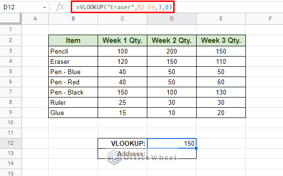
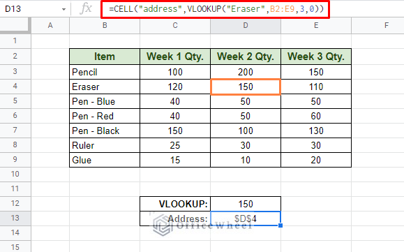
To show the process, we have created the following worksheet where a VLOOKUP formula is used to extract the number of Erasers stored for Week 2.
=VLOOKUP("Eraser",B2:E9,3,0)Now to find the address of our lookup match, we will utilize the CELL function.
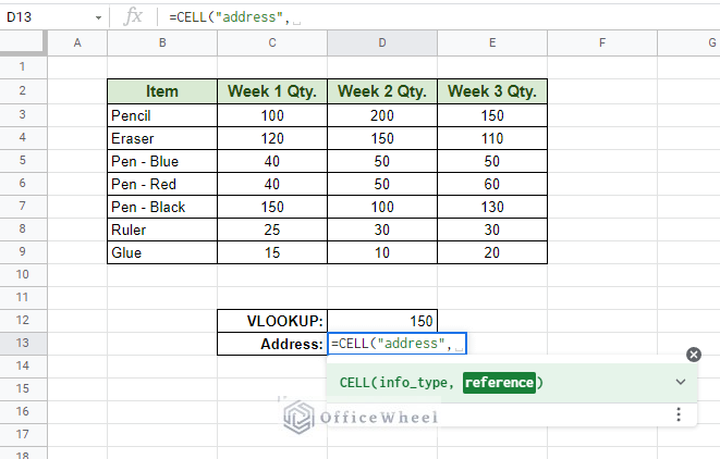
We begin by applying the “address” clause to the formula:
=CELL("address",
The reference section will be covered by the VLOOKUP function used to extract our information. Thus, the final formula looks something like this:
=CELL("address",VLOOKUP("Eraser",B2:E9,3,0))We have successfully found the cell reference of the result of the VLOOKUP data in Google Sheets.
Read More: Combine VLOOKUP and HLOOKUP Functions in Google Sheets
Alternative to VLOOKUP
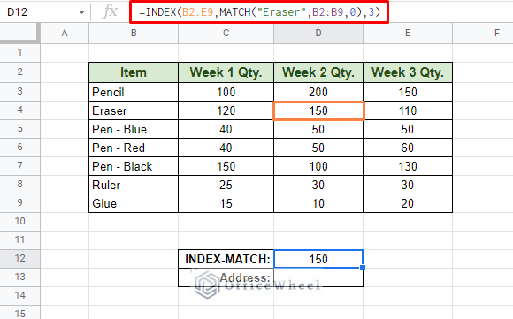
The direct, if not better, alternative to the VLOOKUP function is the INDEX-MATCH formula.
We achieve the same results with the INDEX-MATCH combination in our worksheet:
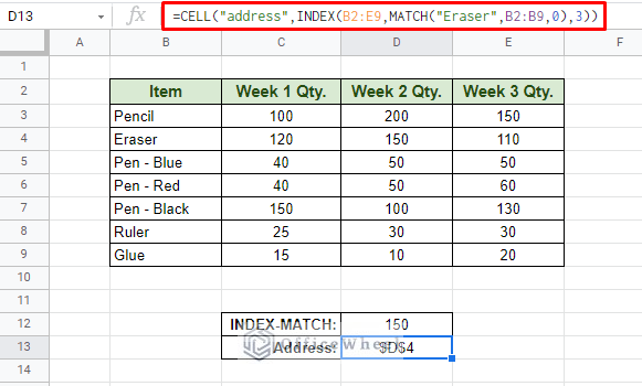
Like before, we simply replace the reference section of the CELL function with the INDEX-MATCH formula:
=CELL("address",INDEX(B2:E9,MATCH("Eraser",B2:B9,0),3))Read More: Alternative to Use VLOOKUP Function in Google Sheets
A More Dynamic Alternative to Find Cell Reference
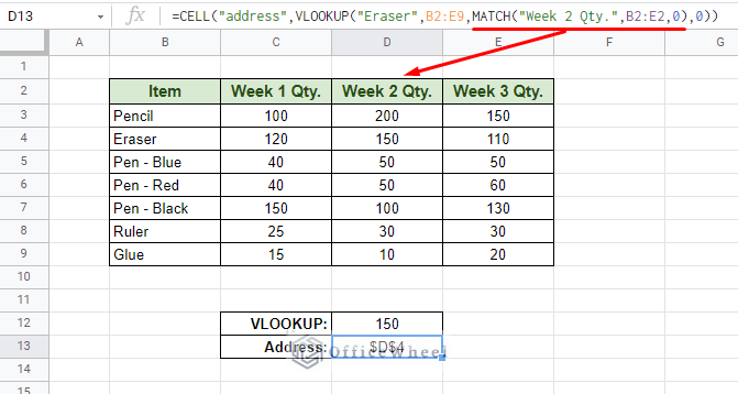
In the last two examples, we had manually inputted the column number of “Week 2 Qty.” in our VLOOKUP and INDEX-MATCH formulas, which was 3.
To make it more intuitive, we will use a MATCH function to determine the column number.
MATCH("Week 2 Qty.",B2:E2,0)In the formula:
=CELL("address",VLOOKUP("Eraser",B2:E9,MATCH("Week 2 Qty.",B2:E2,0),0))We can further our formula by using all the capabilities of Google Sheets to create something truly practical for any size of datasets.
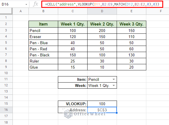
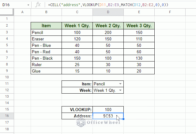
For the following worksheet, we have used more cell references in our formula and drop-down menus to determine our search conditions:
The formula:
=CELL("address",VLOOKUP(D11,B2:E9,MATCH(D12,B2:E2,0),0))And our worksheet in action:
Read More: Lock Cell Reference in Google Sheets (3 Ways)
Final Words
The need to find a cell reference in Google Sheets may not be a common occurrence, but it is definitely a technique that may come in handy for many organizational tasks, especially when you are working with a large dataset.
Please feel free to leave any queries or advice you might have for us in the comments section below, or go through the other related topics we have just for you.
Related Articles
- Return Cell Reference in Google Sheets (4 Easy Ways)
- How to Query Cell Reference in Google Sheets
- Dynamic Cell Reference in Google Sheets (Easy Examples)
- Relative Cell Reference in Google Sheets
- Cell Reference From String in Google Sheets
- Google Sheets: Use Cell Value in a Formula (2 Ways)
- Reference Cell in Another Sheet in Google Sheets (3 Ways)
- How to Create Conditional Drop Down List in Google Sheets

