Dynamic Cell Reference in Google Sheets (Easy Examples)

Today, we will go through an in-depth guide of how to use a dynamic cell reference in Google Sheets, for both within the same worksheet or reference cells from different worksheets.

Let’s get started.

The Core of Our Topic: The INDIRECT function

The fundamental function we will use to dynamically reference cells is the INDIRECT function.

The syntax:

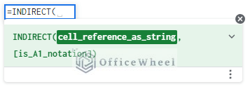
• cell_reference_as_string: The references of the cell or cells are inputted as a string. Any combination of columns and rows can be used.
• [is_A1_notation]: Optional. By default, it is TRUE. Indicates if the reference is in A1 form (COLUMN-ROW) or R1C1 form (ROW-COLUMN).

Volatility of INDIRECT

It is a heavyweight calculation function that can eat up a lot of resources if not used with proper understanding.

Every time the workbook re-calculates, the INDIRECT function re-calculates with it in whichever worksheet it is in. So, your workbook speed might be impacted if you have too many of these functions, especially if you are running on an already resource-heavy browser like Chrome.

Dynamic Cell Reference in the Same Worksheet in Google Sheets

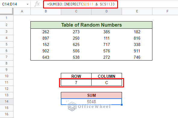
We have created the following table to show our first method of dynamic cell reference in Google Sheets:

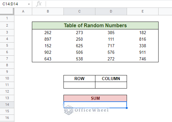
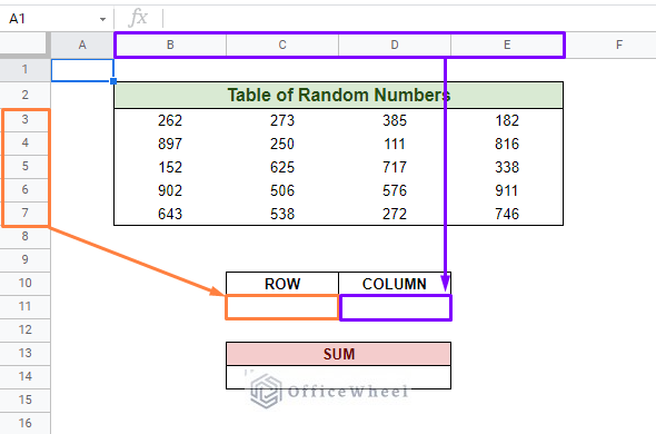
The idea is simple: we will sum the numbers starting from cell B3 up to another cell within the table, which will be dynamically inputted. The target cell reference will be dynamically pulled from the ROW (C11) and COLUMN (D11) cells located below the number table.

Note: Summations can be done in multiple ways in a spreadsheet. The purpose of this method is just to show you how to reference cells dynamically.

Now, in our SUM cell, cell C14, we input the following formula:

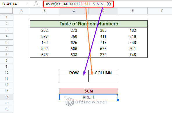
We get a reference error (#REF!) because our reference cells are empty.

Formula Breakdown:

• SUM: The basic sum function for Google Sheets. SUM(B3: is our starting point.
• INDIRECT($D$11 & $C$10): Our ending point of the SUM function. Dynamically references the COLUMN number ($D$11) and the ROW number ($C$10). These references are locked in place by absolutes ($).

Let’s say we want to sum the range B3:C7, we simply add the column and row references in the COLUMN (C) and ROW (7) cells. Our result:

You can input any cell reference with the table:

This concludes the general way to use a dynamic cell reference in Google Sheets. You can see more examples just below to get a better understanding.

Another Example: Sum by Row

We will now see another take of the SUM with the dynamic cell reference method we worked with previously. This time, we will add the ROW function to it.

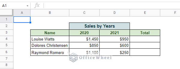
In the following table, we will sum the total sales achieved by each employee over the years 2020 and 2021. We will do this for each row.

Our formula for each row:

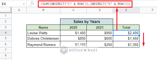
Formula Breakdown:

• ROW(): We have kept it blank so that it returns the immediate row number of the cell it is in. E.g., if the function is in row number 4, it will return 4.
• INDIRECT(“D” & ROW()): Simply refers to column D and current the row number of the cell this function is in.
• SUM: The basic SUM function of Google Sheets. Adds its contents.

Read More: Google Sheets: Use Cell Value in a Formula (2 Ways)

Dynamic Cell Reference in a Different Worksheet in Google Sheets

The more common scenario where we need to dynamically reference cells is when referencing cells from another worksheet in Google Sheet. This is where the INDIRECT function truly shines.

For this example, we will use the following dataset. Here, the Expenses column dynamically references another cell in both the current and another worksheet by the Month name.

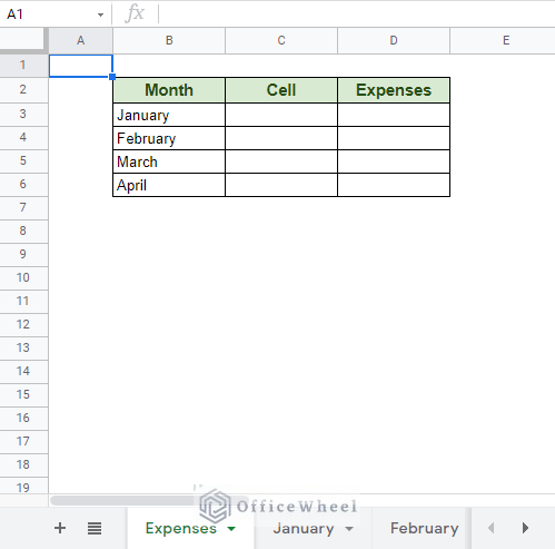
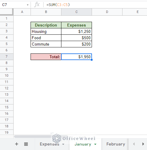
In the other Month worksheet, we have the individual expenses and the total on cell C7. It is the case for all Month worksheets for simplicity.

Thus, in the Expenses worksheet, the Cell column will have C7 in all the cells. And in cell D7 is where we input our formula:

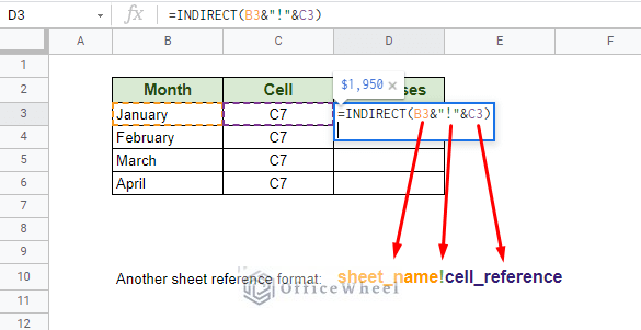
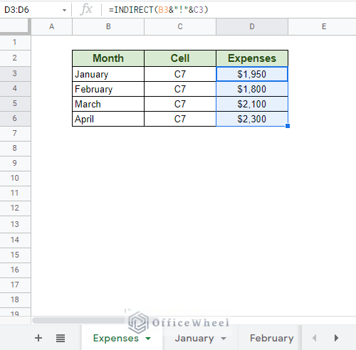
The result after applying to the rest of the column:

Using Dynamic Named Ranges

The dynamic named range is perhaps the best way to organize multiple ranges of cells in a workbook. For this article, dynamic named ranges will give us an easy way to reference a range of cells from another worksheet easily.

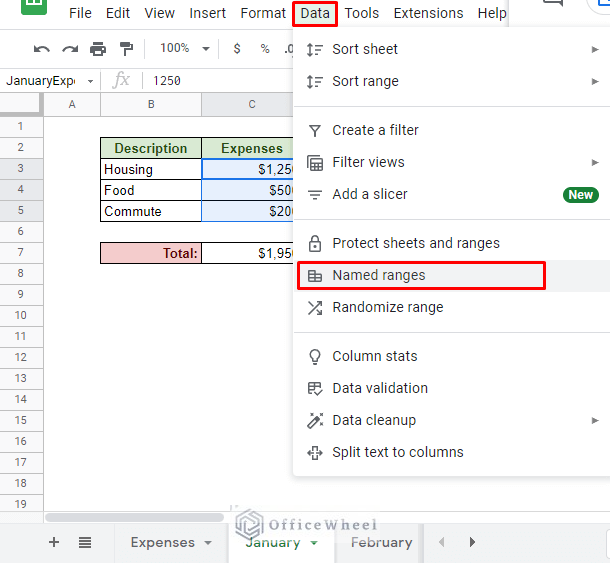
To apply a named range in a Google Spreadsheet, simply select the range of cells you want to name and navigate to Named ranges from the Data tab.

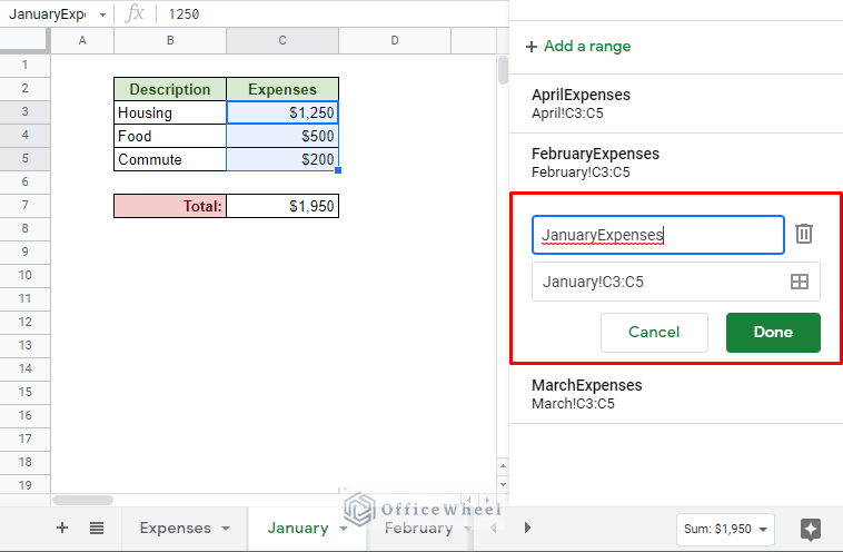
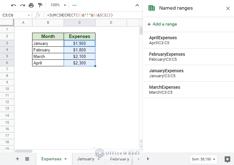
For example, we have named our January worksheet’s Expenses column as “JanuaryExpenses”. The same goes for the rest of the month worksheets.

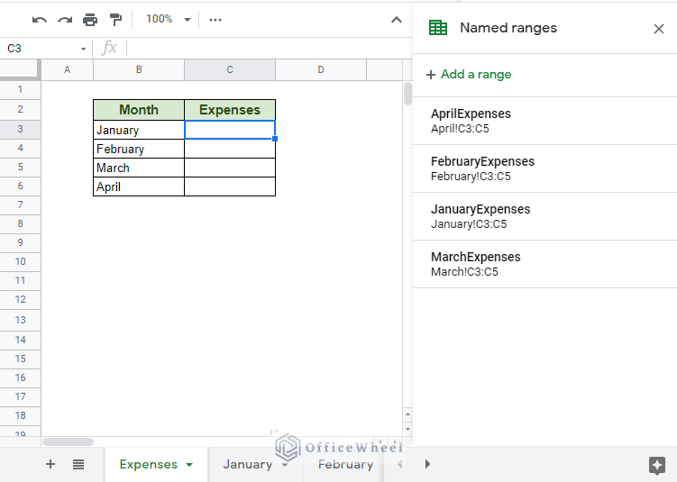
Back in our Expenses worksheet, we have removed the Cell column as we will not need it anymore with this method. Our new formula will take only three cell references that can be already found from the current table.

Our new formula:

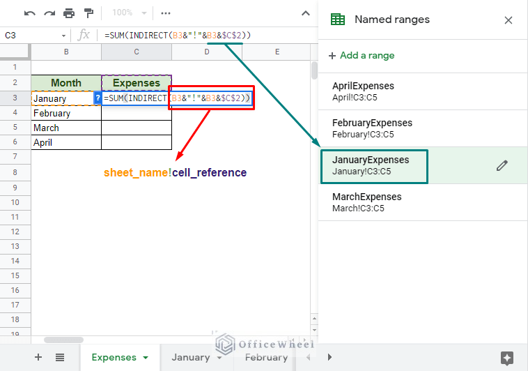
Notice that the cell_reference itself is the Named Range, where the word “January” is taken from cell B3 and the word “Expenses” is taken from cell C2 (it is locked by absolutes ($) as there is only one reference for all the rows).

We have used the SUM function to get the total expenses.

Applying the formula to the rest of the column:

Read More: Reference Cell in Another Sheet in Google Sheets (3 Ways)

Final Words

Knowing how to use a dynamic cell reference in Google Sheets is a must for any aspiring Google Sheets expert. These methods, for both within the same worksheet or beyond it, can come in handy when organizing large amounts of data.

Please feel free to leave any queries or advice you might have for us in the comments section below.

Related Articles

• Reference Another Workbook in Google Sheets (Step-by-Step)
• How to Query Cell Reference in Google Sheets
• Variable Cell Reference in Google Sheets (3 Examples)
• Cell Reference From String in Google Sheets
• Reference Another Sheet in Google Sheets (4 Easy Ways)
• Lock Cell Reference in Google Sheets (3 Ways)