Today, we will look at the different scenarios where we use a variable cell reference in Google Sheets. While the idea is simple, utilizing it can get quite complex when we utilize it for professional-level spreadsheets.
Let’s get started.
3 Ways to Work With Variable Cell Reference in Google Sheets
1. Basic Variable Cell Reference: Locked Cells ($)
As a beginner, the first instance of variable cell reference you will get is by using the fill handle of any spreadsheet application.
Using the fill handle generates values automatically following the pattern of your selected data.
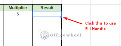
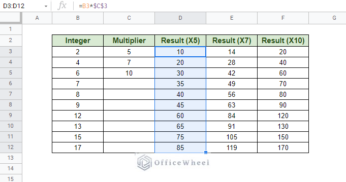
The magic happens when you use it on a formula that uses cell references. To show that, let’s multiply a bunch of integers, however, we have only one multiplier, 5.
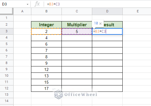
Now, if we apply the formula to the rest of the column with the fill handle, we will not get the desired result. Because the cell reference of the Multiplier is also changing (varying) with each new row.
What we have here, for both Integer and Multiplier, is that they are variable cell references down the column. To keep one column constant (multiplier), we must lock the cell reference in place. We do that by using absolutes ($) in front of both the column and row numbers.
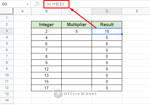
Applying this format to the rest of the column with fill handle:
Read More: Lock Cell Reference in Google Sheets (3 Ways)
2. Using INDIRECT to Extract User-Defined Variable Cell Reference
When we think about variable cell references, we can also think about user-defined cell references. That is when a cell reference changes according to user input.
While no general function in Google Sheets can take a variable cell reference like that, we can overcome this limitation by using the INDIRECT function.
INDIRECT function syntax:
INDIRECT(cell_reference_as_string, [is_A1_notation])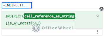
In the following worksheet, we are going to define the Column and Row number of the cell whose data we want to extract (from the Result column)
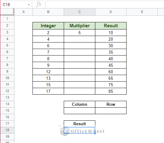
Let’s say we want to extract the value from cell D10. In the Column section, we input “D” and in the Row section we input 10. As for the formula:
=INDIRECT(C15&D15)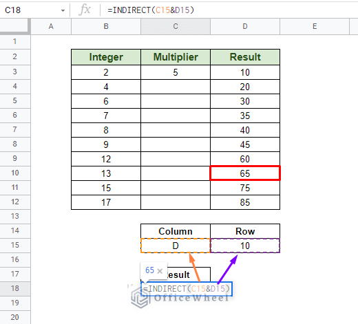
Why this works as a variable cell reference is that we can change the values of the Column and Row numbers anytime.
Read More: Dynamic Cell Reference in Google Sheets (Easy Examples)
Similar Readings
- Indirect Range in Google Sheets (3 Easy Ways)
- Reference Cell in Another Sheet in Google Sheets (3 Ways)
3. Using Named Range as Variable Cell Reference
Another way to work with variables in Google Sheets is to apply names to cell ranges via Named Range.
Steps to apply a Named Range
Step 1: Select the range of cells that you are looking to name.
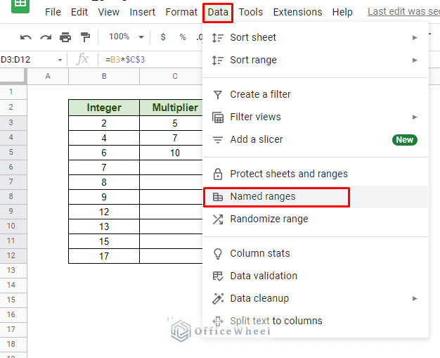
Step 2: Navigate to the Named ranges option from the Data tab. Data > Named Ranges
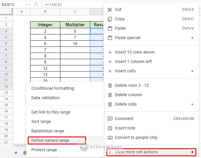
Or, by right-clicking over the selection and selecting the Define named range option. Right-Click > View more cell actions > Define named range
Step 3: In the Named ranges menu, input the name that you want your selected range to be called. Click Done when you are finished.
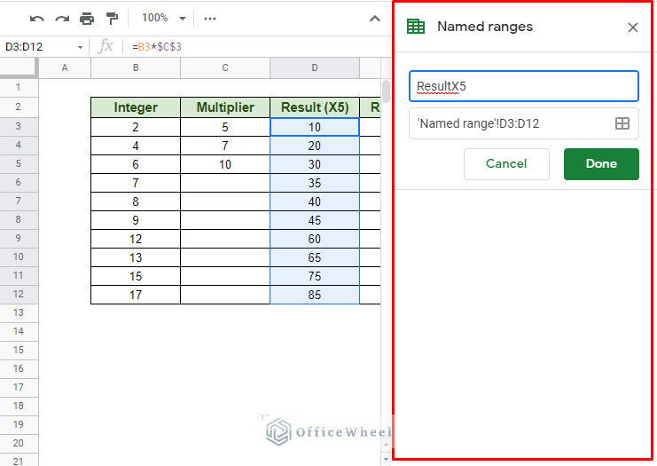
We have applied a named range for each of the Result columns.
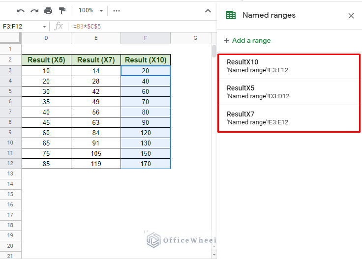
The purpose of this setup is to call each named range to act as a variable in our formula. Our task is to simply find the total of each result column.
For example, we have named the values in the Result (X5) column to be ResultX5. So, we can simply have the SUM formula:
=SUM(ResultX5)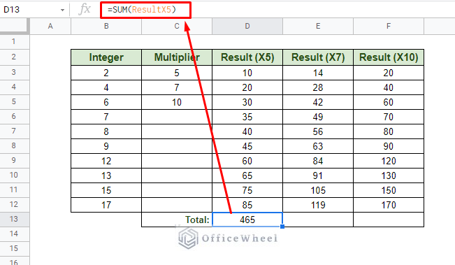
The same can be done for the other two columns:
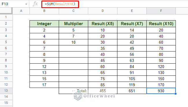
We can even use all ranged names in a single formula:
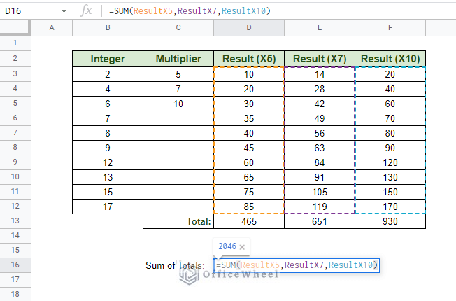
The possibilities are endless when we use named ranges as variables.
Extra: Combining Ranged Names and INDIRECT for Variable Cell Reference in Google Sheets
Since the INDIRECT function takes a string as its value, we can use ii in other formulas by taking string values from user-defined cells.
For example, here we have a worksheet where there is a drop-down list of all the named ranges. These values are obviously text and cannot be utilized in a regular function.
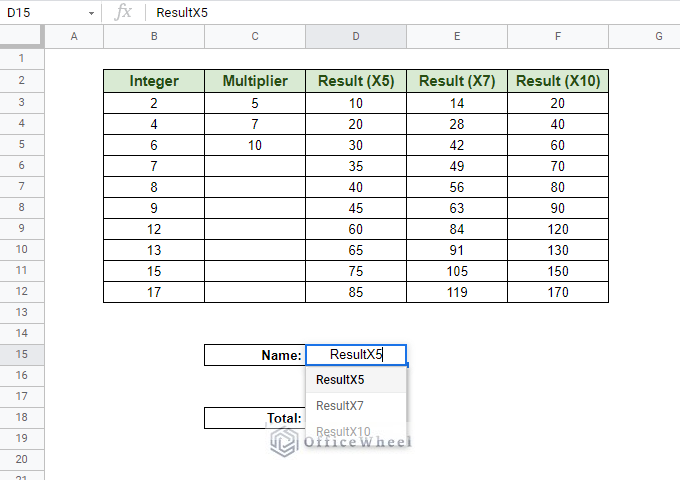
Now, if we put the following formula down:
Read More: Indirect Sheet Name in Google Sheets (Easy Steps)
Final Words
In this article, we have seen the few basic to complex ways in which we can use a variable cell reference in Google Sheets. Know that we’ve only touched on a few examples and many more iterations of what we have discussed are out there to be discovered, especially with Named Ranges, INDIRECT, or even QUERY. So, go ahead and take these ideas on a test drive.
Please feel free to leave any queries or advice you might have for us in the comments section below.
Related Articles
- Reference Another Sheet in Google Sheets (4 Easy Ways)
- Google Sheets: Use Cell Value in a Formula (2 Ways)
- Relative Cell Reference in Google Sheets
- Reference Another Workbook in Google Sheets (Step-by-Step)
- Cell Reference From String in Google Sheets
- Find Cell Reference in Google Sheets (2 Ways)
- Reference Another Tab in Google Sheets (2 Examples)