Average is the most useful parameter for any business calculation. Sometimes it requires entering new data and averaging with the newest entry to find the current trend or pattern. In this article, we discuss three quick solutions along with their alternative in cases to find the average of the last N rows in Google Sheets.
A Sample of Practice Spreadsheet
You can download the spreadsheets from the link below. After downloading you can practice on your own as we demonstrate in this article.
3 Suitable Ways to Calculate Average of Last N Rows in Google Sheets
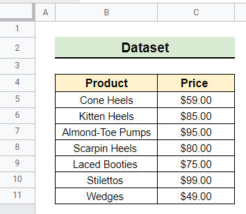
First, we have to give a look at the dataset. In the dataset, prices of different products are given. We want to average the last N rows of the Price column. Here, N is the number of cells we want to average.
1. Using OFFSET and AVERAGE Functions
The aggregation of AVERAGE, COUNT and OFFSET functions can perform the task of averaging the last N rows in Google Sheets. The OFFSET function is used to find the range that needs to average. In this solution, we want to average the last 3 rows of the Price column.
Steps:
- First, we select the cell in which we want to show the average of the last N rows. Here, we select cell E5 to show the average of the last 3 rows.
=AVERAGE(OFFSET(C5, COUNT(C5:C)-3,0,3))- Then we insert the above formula in the formula bar.
- Finally, the output is shown in the selected cell. By tweaking the formula to suit your needs, you can get the average of the last N number of rows.
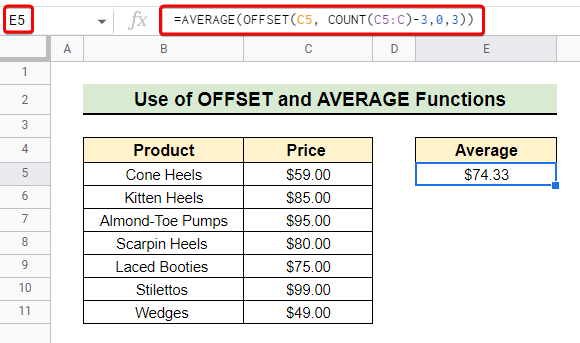
Formula Breakdown First, the COUNT function counts the numeric entries of the entire column C from cell C5. Then, the OFFSET function returns the last three rows with entries. Finally, the AVERAGE function averages the last three rows.
Alternative Solution
An alternative solution using the OFFSET function is below. You may try it if you find it easier.
Steps:
=IFERROR(AVERAGE(OFFSET($C$5,MAX(0, COUNT($C$5:C)-3),0,3,1)),0)- First, we have to insert the above formula in the formula bar as earlier.
- Then we hit Enter to get the desired output of getting the average of the last 3 rows. You can change the row number based on your dataset to get the desired average.
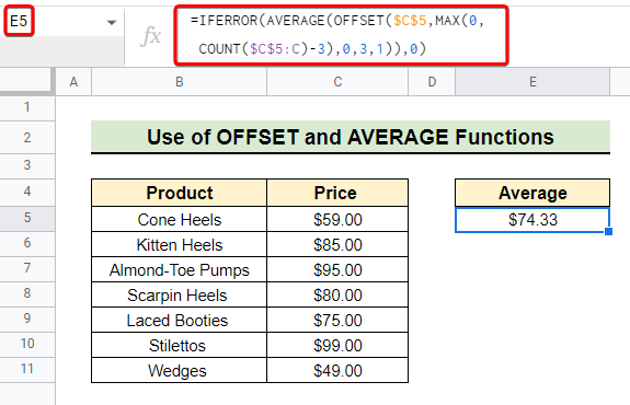
First of all, the COUNT function counts the numeric entries of the entire column C from cell C5. Then, the MAX function returns zero if the return of the COUNT function is less than three. This means there are not enough numeric entries to average last three rows. Next, the OFFSET function returns the last three entries. Afterward, the AVERAGE function calculates the average of last three rows. Finally, the IFERROR function returns its second argument zero if there is any error in calculating the average.
Read More: How to Average Cells from Different Sheets in Google Sheets
2. Applying SORT and QUERY Functions
SORT and QUERY functions along with some other functions can also find the range of the last N rows for averaging in Google Sheets. The SORT function sorts rows by column and the QUERY function runs Google Visualization API QUERY Language query.
Steps:
- At first, we select the cell in which we want to show the average of the last N rows. Here, we select cell E5 to show the average of the last 4 rows.
=ARRAYFORMULA(AVERAGE(QUERY(SORT(C5:C,ROW(C5:C)* ISNUMBER(C5:C),FALSE), "limit 4",0)))- Then we insert the above formula in the formula bar to get the average of the last 4 rows.
- Finally, the output is shown in the selected cell. You can alter the number of rows by modifying the formula to suit your needs.
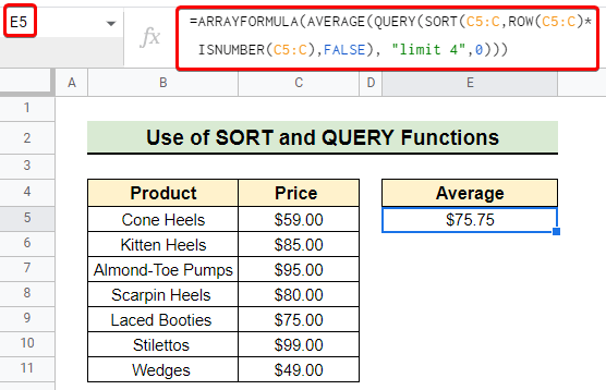
Formula Breakdown Initially, the ROW function returns the numeric value of the first row. In our case, the numeric value of the first row is 5 as C5 is at row 5. The ISNUMBER function returns TRUE if a cell contains a numeric entry. Otherwise, it returns FALSE. It passes as an argument of the SORT function. Then, the SORT function sorts the range in descending order. Next, the QUERY function returns the last four numeric entries. The AVERAGE function averages the last four numeric entries. Finally, the ARRAYFORMULA returns the single output of the average in the selected cell by taking the formula within it as an array formula. If we don’t use ARRAYFORMULA it also works perfectly.
Read More: How to Add Average Line in Google Sheets (With Detailed Steps)
3. Utilizing FILTER and AVERAGE Functions
The FILTER function can be very useful in finding the range of the last N rows. In the following solution, we use the FILTER function together with the AVERAGE function to get the average of the last four rows.
Steps:
- First, we select the cell in which we want the average of the last N rows. Here, we select cell E5 to show the average of the last 4 rows.
=AVERAGE(INDIRECT("C" & IFERROR(LARGE(FILTER(ROW(C5:C), LEN(C5:C)), 4), ROW(C5)) & ":C")- Then we insert the above formula in the formula bar to get the average of the last 4 rows.
- Finally, we get the average of the last four rows in the selected cell. You can modify the formula and change the number of rows for averaging the last N rows in Google Sheets.
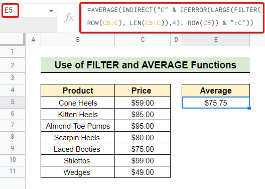
Formula Breakdown Initially, the ROW function returns the numeric value of the first row. In our case, the numeric value of the first row is 5 as C5 is at row 5. Then, the LEN function returns the length of the string of column C from cell C5 to the entire column. Afterward, the FILTER function filters the row numbers of the nonempty entries within the range of C5:C Next, the LARGE function returns the 4 largest row numbers. The IFERROR function is used as a safeguard in the above formula. If there are fewer than four non-empty rows then it begins averaging from the cell C5. Then, the INDIRECT function forms the range of averaging which is the last four entries of this case. At last, the AVERAGE function does the averaging.
Things to Remember
- Make sure you customize the solutions as your need to get the average of the last N rows.
- The first two solutions don’t require numeric entries in the last N rows. These two will always give you the average of the last N numeric entries regardless of their row number.
- The third solution needs numeric entries in the last N rows. Make sure of that.
Conclusion
So these are some ways to calculate the average of the last n rows in Google Sheets. I hope the solutions may help you to get your job done. Further, if you face any trouble in modifying the solutions feel free to comment below and I will try to reach out to you soon. You can also visit our website OfficeWheel for the most useful articles.