The AVERAGE function is one of the basic and useful functions in Google Sheets. It helps the users to get an arithmetic mean of a set of numerical values. You can calculate the average of values or a range of cells in Google Sheets. In this article, we will explain the anatomy of this function and a few suitable examples of how to use the AVERAGE function in Google Sheets.
A Sample of Practice Spreadsheet
You can download the practice spreadsheet from the download button below.
What Is AVERAGE Function in Google Sheets?
The AVERAGE function returns the arithmetic mean of a set of numerical values.
Syntax
The Syntax of the AVERAGE function is shown below.
AVERAGE(value1, [value2, …]) 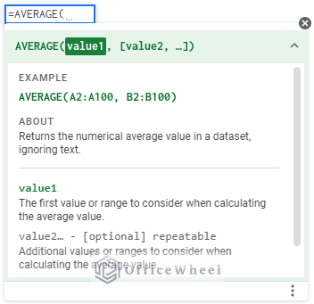
Arguments
| ARGUMENT | REQUIREMENT | Function |
|---|---|---|
| value1 | Required | The first value or range to consider when calculating the average value. |
| value2 | Optional | Additional values or ranges to consider when calculating the average value. |
Output
The formula AVERAGE(1,2,3) will return 2 because the arithmetic average of these three values is 2.
4 Suitable Examples of Using AVERAGE Function in Google Sheets
There are various ways you can find averages from a dataset using the AVERAGE function.
Suppose, you have a dataset that contains the monthly salary of some employees of a company in the first three months of a particular year.
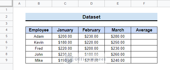
You can find the average salary for each person using the AVERAGE function.
Here, you can find averages in multiple ways in a dataset. You can use the cell values, and range of cells or combine both of them.
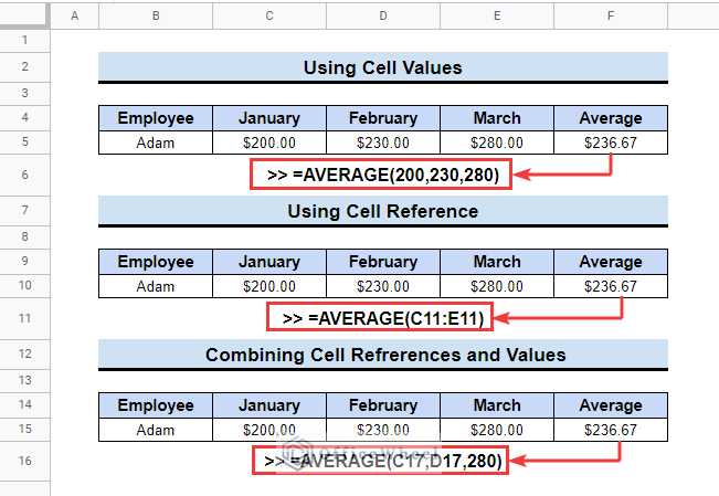
1. Using Cell Values
You can easily find the average of some numerical values using the AVERAGE function. This is a very simple thing to do. Now we will find the average using some direct values from the dataset. Follow the steps below to learn how to do that.
📌 Steps:
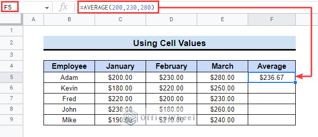
- At the very beginning, select cell F5 in the dataset.
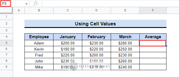
- Subsequently, to find the salary average of Adam, insert the following formula.
=AVERAGE(200,230,280)- Following, hit the Enter key.
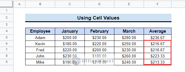
- After that, input the respective values of other employees similarly.
- Finally, you will get the averages for all the employees.
Read More: How to Average Cells from Different Sheets in Google Sheets
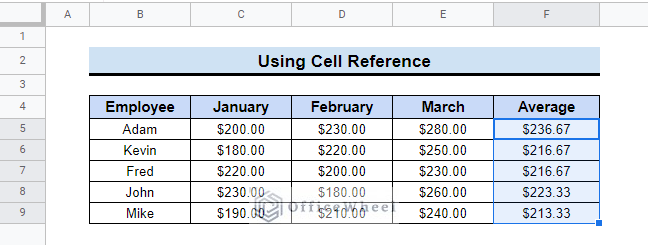
2. Using Cell Reference
Now, we have put the direct values in some cells. Besides, we can find the averages using cell references. Please read along furthermore to learn how to do that by yourself.
📌 Steps:
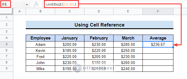
- First, select cell F5 and insert the following formula in the formula bar.
=AVERAGE(C5:E5)- Subsequently, press the Enter key.
- Next, drag down the fill handle tool to copy the formula similar to other relevant cells.
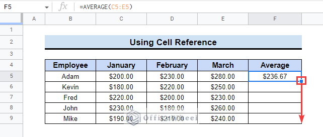
- Finally, you will see the average of the next relevant cells.
Read More: Calculate Average of Last N Rows in Google Sheets (3 Ways)
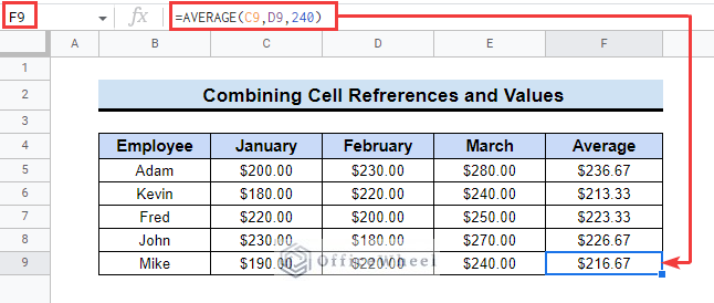
3. Combining Values and Cell References
Moreover, you can also find the averages combining direct values and cell references. At this time, we will use the AVERAGE function and put both the values and cell references in it. Follow the next steps and you can also do that.
📌 Steps:
- First, enter the following formula in cell F5.
=AVERAGE(C5,D5,280)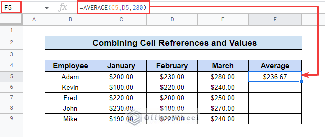
- Then, you will get the average in that cell.
- Similarly, you can select specific cells and add values to find the average for other cells similarly.
Read More: How to Add Average Line in Google Sheets (With Detailed Steps)
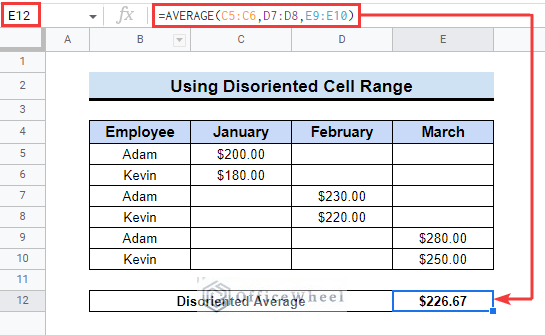
4. Using Disoriented Cell Ranges
Furthermore, if you need to find the average of some disoriented cell ranges in a dataset, that can also be done using the AVERAGE function.
For example, here is a dataset where the salary of Adam and Kevin are given for 3 consecutive months. Following, their January salaries are mentioned respectively in cells C5 and C6, February salaries in cells D7 and D8, and finally their salaries for March are subsequently in cells E9 and E10.
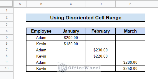
You need to find the average of their salary. Read the below steps to learn that.
📌 Steps:
- First, select the cell E12 and enter the below-mentioned formula.
=AVERAGE(C5:C6,D7:D8,E9:E10)- Following, hit the Enter key.
- Next, the average will be in the selected cell.
Things to Remember
- The AVERAGE function ignores texts and boolean values(TRUE/FALSE).
- The AVERAGE function ignores blank cells but includes a cell containing zero value.
Conclusion
So, in this article, we have tried to show you how to use the AVERAGE function in Google Sheets. Hopefully, the methods above will be enough for you to understand the applications of the function. Besides, please use the comment section below for further queries or suggestions. You may also visit our OfficeWheel blog to explore more about Google Sheets.