We average our data often in Google Sheets. However, when we average our data, we may find blank cells. While averaging our data, we may want to omit those blank cells in the data range. In this article, I’ll demonstrate 5 simple ways to ignore the blank cells while using the AVERAGE formula in Google Sheets.
5 Simple Ways to Ignore Blank Cells with AVERAGE Formula in Google Sheets
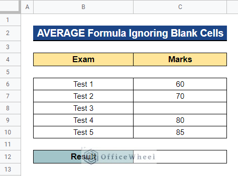
We will use the dataset below to demonstrate 5 simple ways to ignore the blank cells while using the AVERAGE formula in Google Sheets. The dataset contains an exam list and a student’s exam marks. And we want to find the student’s average marks while there is a blank cell in the marks list.
1. Using AVERAGE Function
The AVERAGE function excludes blank cells and cells with text values by default. As a result, no extra procedures are required to average your data while disregarding blanks and text items in the data range.
Steps:
- Firstly, select the cell where you’re going to apply the formula. In our case, we selected Cell C12. Next, enter the formula below and press Enter–
=AVERAGE(C6:C10)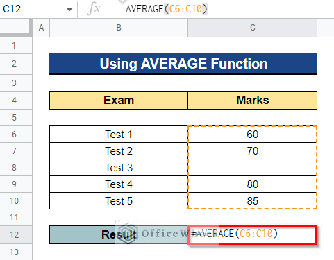
- Thus, you will get the average marks received by the student.
![]()
Read More: How to Average Cells from Different Sheets in Google Sheets
2. Applying AVERAGEIF Function
The AVERAGEIF function, like the AVERAGE function, eliminates blank cells and cells with text values by default. As a consequence, no additional procedures are necessary to average your data while disregarding blanks and text items in the range. However, in cases when cells include zeros, you must use the AVERAGEIF function with the constraint Not Equal to Zero.
Steps:
- First, choose the cell where you want to apply the formula. In our situation, we chose Cell C12. Next, input the following formula and hit Enter–
=AVERAGEIF(C6:C10,"<>0)")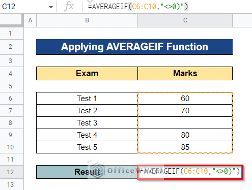
- As a result, you will obtain the student’s average grade.
![]()
3. Joining IF, COUNT, and AVERAGE Functions
In Google Sheets, you may determine the average value of a range by combining the IF, COUNT, and AVERAGE Functions, but only if all cells in the range are not blank. If all of the values in the range are blank, this method returns 0.
Steps:
- First, choose the cell to which you want to put the formula. Cell C12 was chosen for our situation. Next, input the formula below and hit Enter–
=IF(COUNT(C6:C10),AVERAGE(C6:C10),0)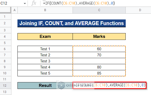
Formula Breakdown
- COUNT(C6:C10)
First, the COUNT function just counts the numeric values in Cell C6:C10.
- AVERAGE(C6:C10)
The AVERAGE function then gives the numerical average value in the Cell C6:C10 range.
- IF(COUNT(C6:C10),AVERAGE(C6:C10),0)
Finally, the IF function averages the cells counted by the COUNT function in the data range Cell C6:C10.
- Therefore, you will obtain the student’s average marks.
![]()
Read More: Calculate Average of Last N Rows in Google Sheets (3 Ways)
4. Combining SUMIF and COUNTIF Functions
We can even utilize the SUMIF and COUNTIF functions together in Google Sheets to get the average value of a range while disregarding blank cells and cells containing 0.
Steps:
- First, choose the cell where you want to use the formula. In this example, we chose Cell C12. Then, input the following formula and hit Enter–
=SUMIF(C6:C10, "<>0")/ COUNTIF(C5:C10, "<>0")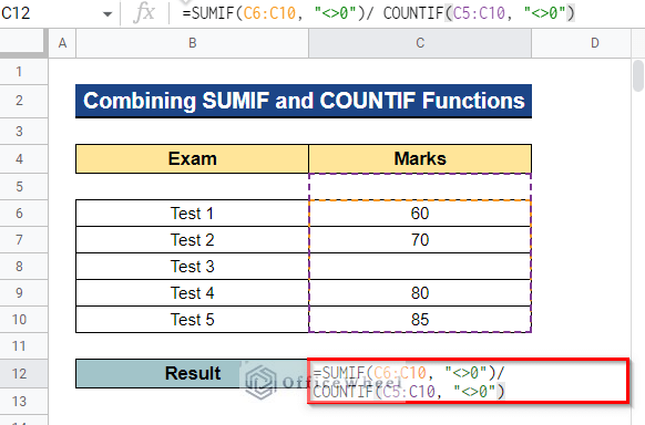
Formula Breakdown
- SUMIF(C6:C10, “<>0”)
The SUMIF function sums all the numeric cells which have a value greater than or less than 0 in the range Cell C6:C10.
- COUNTIF(C5:C10, “<>0”)
And, the COUNTIF function counts any numeric cells in the range Cell C6:C10 that have a value higher than or less than 0.
- As a result, you will have the average marks of the students.
![]()
5. Merging AVERAGE.WEIGHTED, FILTER, and ISNUMBER Functions
With the values and the accompanying weights, we can use the AVERAGE.WEIGHTED function to get the weighted average of a group of values. However, if there are any blank cells in the data range, it will display a red error notice. To determine the weighted average while disregarding the blank cells, we must combine the AVERAGE.WEIGHTED, FILTER, and ISNUMBER functions.
Steps:
- Firstly, choose the cell where you want to execute the formula. In our case, we chose Cell C12. Next, input the following formula and push Enter–
=AVERAGE.WEIGHTED(FILTER(C6:C10,ISNUMBER(C6:C10)),FILTER(D6:D10,ISNUMBER(C6:C10)))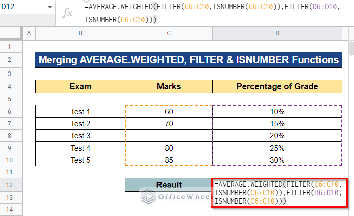
Formula Breakdown
- ISNUMBER(C6:C10)
First, the ISNUMBER function determines if the values in Cell C6:C10 are numbers.
- FILTER(C6:C10,ISNUMBER(C6:C10))
The FILTER function then returns all of the numeric values that are checked by the ISNUMBER function to see if they are number values.
- WEIGHTED(FILTER(C6:C10,ISNUMBER(C6:C10)),FILTER(D6:D10,ISNUMBER(C6:C10)))
Finally, the AVERAGE.WEIGHTED function determines the weighted average of the cells.
- Thus, you will get the desired output.
![]()
How to Use AVERAGE Formula to Ignore 0 in Google Sheets
Sometimes we have cells in Google Sheets that contain 0 and we wish to omit those cells while averaging our data. We can accomplish this with the AVERAGEIF function.
Steps:
- To begin, choose the cell to which you wish to apply the formula. In our situation, we chose Cell C12. After that, enter the following formula and hit Enter–
=AVERAGEIF(C6:C10,">0")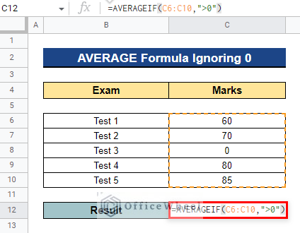
- Therefore, you will get the student’s average marks while ignoring 0 in a cell.
![]()
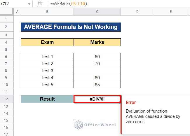
What to Do If AVERAGE Formula Is Not Working in Google Sheets?
When using the AVERAGE function to average your data, you may occasionally receive an error message instead of the average value. Even if you typed the formula correctly, it will not function if your data is in Text format. You have to make sure that all of your data are in Number format.
Steps:
- In Cell C12, we have used the AVERAGE formula to average our data. But as our data are in the wrong format, it’s showing a #DIV/0! error.
- To change the format of the dataset, first select all the cells. In our case, we selected Cell C6:C10. Now, go to the More formats option.
![]()
- Next, select the Number format.
![]()
- Thus, you will get the desired output.
![]()
Conclusion
In this article, I have shown 5 simple ways to ignore the blank cells while using the AVERAGE formula in Google Sheets. I have also shown how to use the AVERAGE Formula ignoring 0 in Google Sheets and what to do if the AVERAGE formula is not working in Google Sheets. I hope this will be helpful. Please feel free to ask any questions or suggest any ideas in the comment section below. To explore more, visit Officewheel.com.