In the financial analysis, we use the moving average as a tool. It is also known as the running average. We can calculate the moving average by taking the arithmetic mean of a given set of data over a specified number of periods. In short, it is the average change in data series over time. This article will show you how to calculate the moving average in Google Sheets.
What Is Moving Average?
The moving average is an indicator that is used in technical analysis of the market trend of the stocks. Calculating the moving average the short-term fluctuation of the stock price is determined and mitigated for a specified time period. The moving average is similar to the normal average but in the case of the moving average, the time period of the average is kept the same while adding new data to the average.
2 Suitable Ways to Calculate Moving Average in Google Sheets
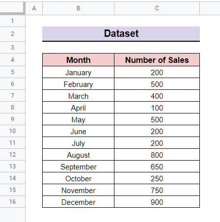
Let’s assume you have a dataset containing monthly sales for an entire year. Now you need to calculate the moving average for every month. You can calculate the moving average in Google Sheets using the AVERAGE function. You can also combine multiple functions to create an array formula to do that. We will use the following dataset to illustrate both of the methods.
1. Using AVERAGE Function
Here we will use the AVERAGE function to calculate the moving averages of the sales in the above dataset. The AVERAGE function returns the average of a given number of numerical values. Follow the steps below to apply the function to calculate the moving average in Google Sheets.
Steps:
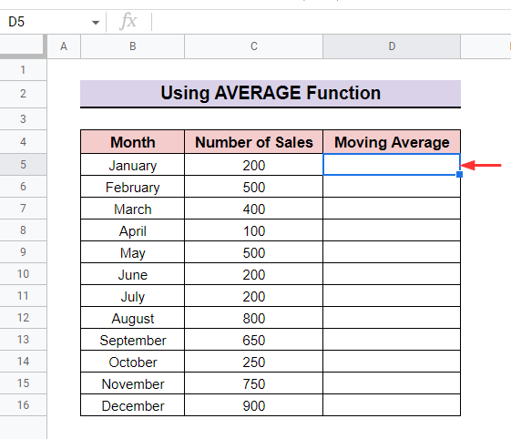
- First of all, create a new column after the sales column and select cell D5 to calculate the moving average.
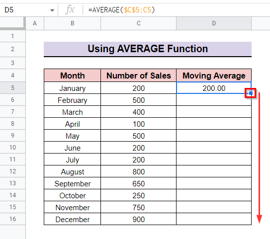
- Then type in the following formula with the AVERAGE function.
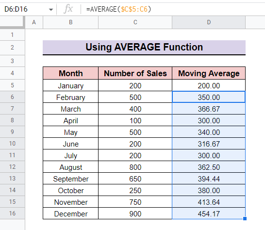
=AVERAGE($C$5:C5)- Next press Enter. The cell will look like the following screenshot. After that, copy the formula to the rest of the cells by dragging the Fill Handle tool.
- In the end, the final output will look like the following screenshot.
Read More: How to Find Average in Google Sheets (8 Easy Ways)
2. Applying ARRAYFORMULA
Here we will create an arrayformula using the SUMIF, COUNTA, and some other functions to calculate the moving average in Google Sheets. The SUMIF function totals the numeric values. Then the COUNTA function returns the denominator to calculate the average.
Steps:
- Enter the following formula in cell D5 to get the same result as earlier.
=ARRAYFORMULA (IF (C5:C16=" ", ,SUMIF (ROW (C5:C16),"<="&ROW (C5:C16),C5:C16)/IFNA (VLOOKUP (ROW (C5:C16),{FILTER (ROW (C5:C16),C5:C16<>" "), SEQUENCE (COUNTA (C5:C16),1)},2,0))))- Finally, the output will look like the following Screenshot.
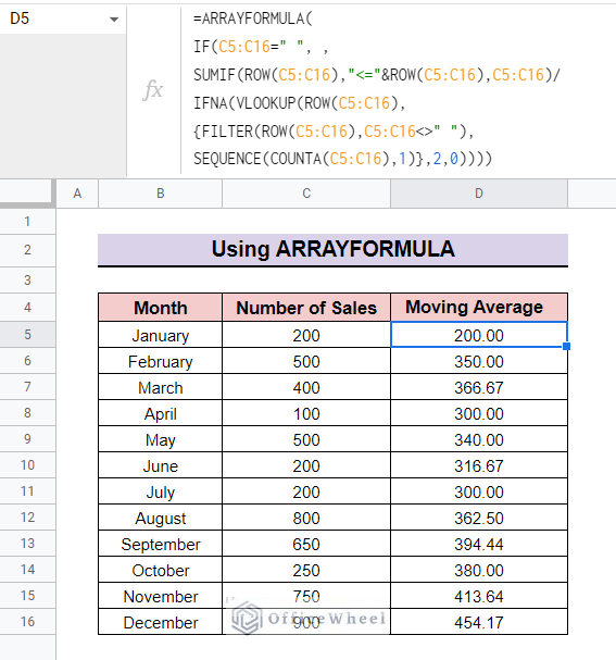
Formula Breakdown The ROW function returns the row numbers of the specified cells. Here, the SUMIF function will return the cumulative sum of the selected cells C5:C16. The IF function returns the output from the SUMIF function only for non-blank cells in the range C5:C16. The COUNTA function returns the non-blank cells within the range C5:C16. Then the SEQUENCE function returns an array of numbers starting from 1 to the number of non-blank cells in that range. Now the FILTER function excludes the row numbers of empty cells. Then the VLOOKUP function looks up values in the filtered array. Next, the IFNA function returns the denominator for the average or an empty string in case of a #N/A error. Lastly, the ARRAYFORMULA will return the moving average by dividing the cumulative sum by the row numbers respectively.
ROW(C5:C16)
SUMIF(ROW(C5:C16),"<="&ROW(C5:C16),C5:C16)
IF(C5:C16=" ", , SUMIF(ROW(C5:C16),"<="&ROW(C5:C16), C5:C16)
COUNTA(C5:C16)
SEQUENCE(COUNTA(C5:C16),1)
FILTER(ROW(C5:C16),C5:C16<>" ")
VLOOKUP(ROW(C5:C16),{FILTER(ROW(C5:C16),C5:C16<>" "), SEQUENCE(COUNTA(C5:C16),1)},2,0)
IFNA(VLOOKUP(ROW(C5:C16),{FILTER(ROW(C5:C16),C5:C16<>" "), SEQUENCE(COUNTA(C5:C16),1)},2,0))
ARRAYFORMULA( IF(C5:C16=" ", , SUMIF(ROW(C5:C16),"<="&ROW(C5:C16), C5:C16)/IFNA(VLOOKUP(ROW(C5:C16),{FILTER(ROW(C5:C16), C5:C16<>" "), SEQUENCE(COUNTA(C5:C16),1)},2,0)) ))
Read More: How to Average Cells from Different Sheets in Google Sheets
Similar Readings
- How to Find 50 Day Moving Average in Google Sheets
- Calculate Weighted Moving Average in Google Sheets
- How to Find 7-Day Moving Average in Google Sheets
How to Calculate Simple Moving Average in Google Sheets
The Simple Moving Average (SMA) calculates the average of a set of data over a selected period of time. It is one of the most frequently used market indicators that indicate the market trend.
Now, to calculate the 3-month Simple Moving Average for the dataset shown above follow the steps below.
Steps:
- In the beginning, select the third cell D7 in the SMA column to calculate the 3-month Simple Moving Average.
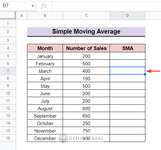
- Then, type the following formula.
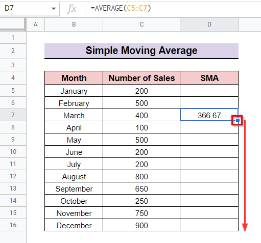
=AVERAGE(C5:C7)- Following that, press Enter. Cell D7 displays the Simple Moving Average for the first three months. After that, for the rest of the cells simply drag the fill handle tool.
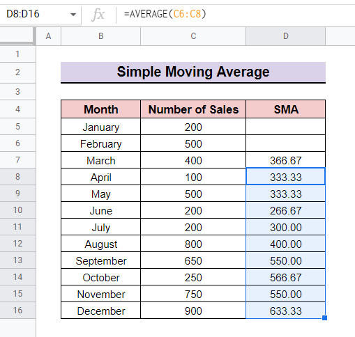
- Finally, you will get the Simple Moving Average for the corresponding cells as follows.
Read More: How to Find 200-Day Moving Average in Google Sheets (2 Ways)
Things to Remember
- While using the average function you have to specify the time period properly to calculate the moving average.
- In case to get the moving average for a specific range you need to define it in the formula because the array formula will return all averages at once according to the entries that are specified in the formula.
Conclusion
These are the ways to calculate the moving average of suitable data. Hopefully, you can easily calculate the moving average following the ways discussed above. Feel free to share your thoughts or comments by reading the article in the comment section. Please visit OfficeWheel for more Google Spreadsheet-related articles.