It is not uncommon that a spreadsheet user may need to apply custom conditions for sorting and organizing data. Understanding that, we will look at how we can apply custom sort in Google Sheets in today’s article.
Let’s get started.
2 Scenarios to Apply Custom Sort in Google Sheets
1. Advanced Sort Range Options
We will be using a basic approach for our first scenario. It is not that different from regular sorting in Google Sheets, only that this time, we will be adding a couple of hierarchical conditions.
This process uses the advanced Sort Range options available to us in Google Sheets.
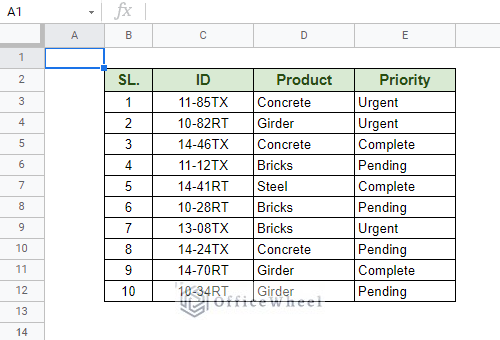
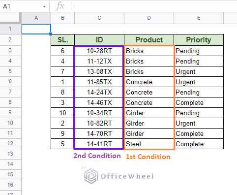
In the following table, we will sort the entries according to these custom conditions in the order of importance:
- Product name
- Product ID
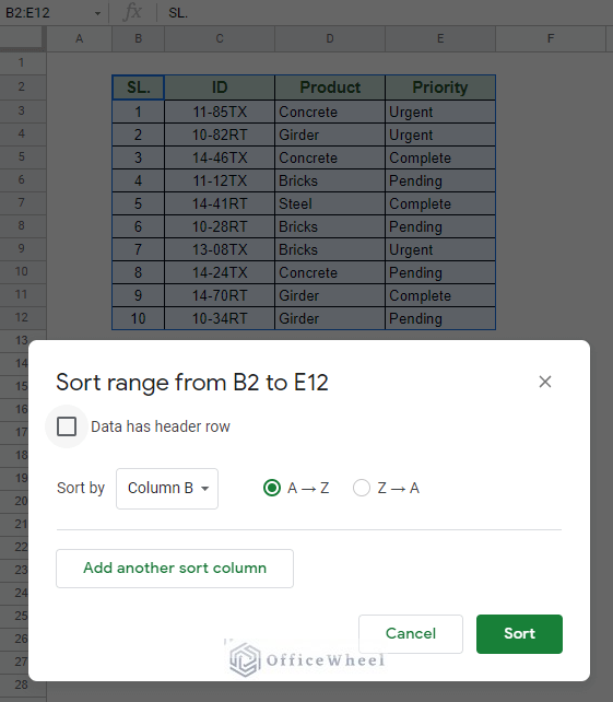
Our first step is to select the whole table (column headers included). Then we open the advanced Sort Range options window. We can do this in two ways:
- Data tab > Sort range > Advanced range sorting options
- Right-click over the selection > View more cell actions > Sort range
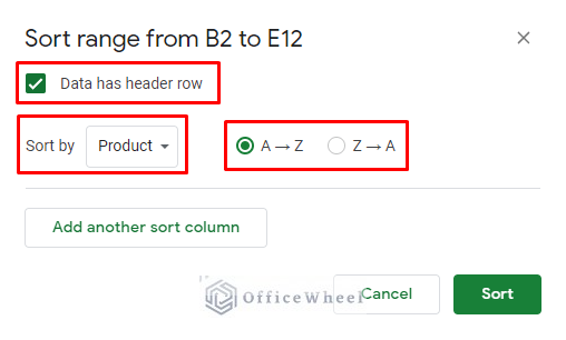
Our first custom sort condition was Product name; thus, we have chosen the following options:
- Check the Data has header row option to open up the header names for column selection (recommended). That is why we suggested that you select the whole table, including the headers.
- Select the Product column for the Sort by option.
- Select A to Z for ascending order.
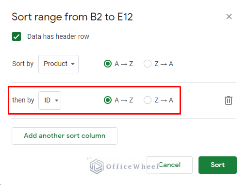
For our next condition, click on the Add another sort column button and select the following options to sort by the ID column:
- Select ID for the then by option. This will add the second column in priority to sort by.
- Select A to Z for ascending order.
Clicking on Sort will sort our table in the custom order we just applied.
That concludes the most fundamental way we can apply conditions to our sort in Google Sheets. To know more about this particular process, please see our How to Sort by Multiple Columns in Google Sheets article.
For a truly customized sorting process, please see the next section of this article.
2. Using a Formula to Custom Sort in Google Sheets
By default, sorting in Google sheets, whether it be numerical or text values, is done traditionally. Value for numbers and alphabetical order for text.
But there is a way to add weight, priority, or value to text to allow us to sort and organize data in a custom order thanks to certain function combinations.
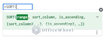
The foundation of our formula will obviously be the SORT function. Its syntax:
We will be combining it with the MATCH function. The MATCH function syntax:
MATCH(search_key, range, [search_type])Our formula and result:
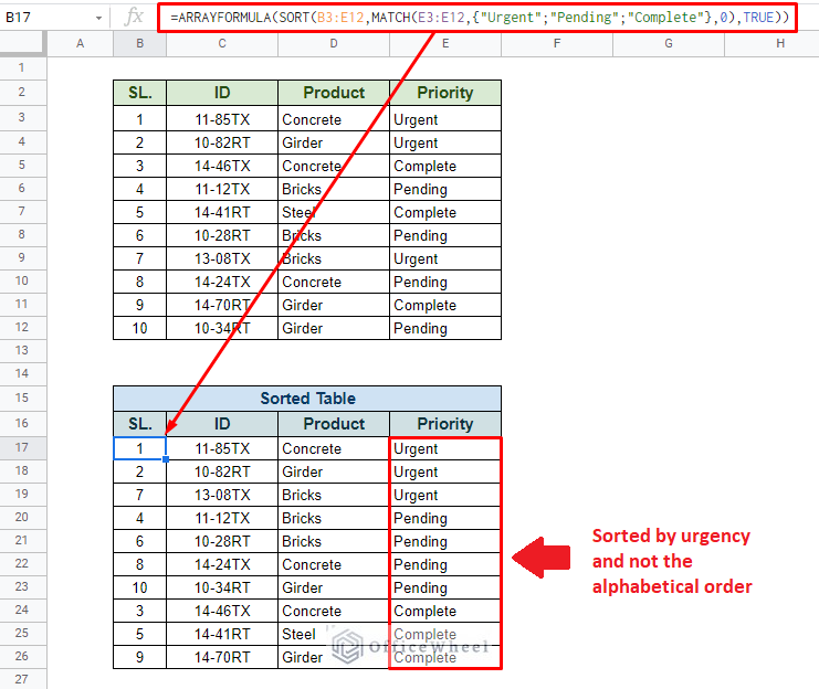
=ARRAYFORMULA(SORT(B3:E12,MATCH(E3:E12,{"Urgent";"Pending";"Complete"},0),TRUE))Formula Breakdown
Let’s do a breakdown of the formula that we have just used. We start with the MATCH formula:
MATCH(E3:E12,{"Urgent";"Pending";"Complete"},0)The MATCH formula is used to generate a column for the SORT function. There are three criteria for the match: Urgent, Pending, and Complete. The leftmost text has the most priority, that is how we determine the hierarchy/value of our sort.
Recall from the MATCH syntax that the function takes only one criterion. Since we have three, we have to input them as an array. Thus, our three text conditions are enclosed in curly braces {} and separated by semicolons (;).
As we have mentioned, the MATCH formula takes the place of the sort_column field of the SORT function (see syntax). For the other fields, we have kept things simple.
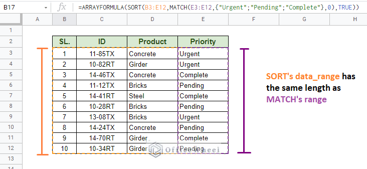
The data_range will obviously be all the value cells within the table. IMPORTANT: It is crucial to make sure that the length of the column of data_range is the same as the range in the MATCH function. This is because our sort_column field value can come from beyond this table.
Finally, since we are working with arrays, we have to enclose the SORT-MATCH formula within ARRAYFORMULA to present the results properly.
Read More: How to Use IF and OR Formula in Google Sheets (2 Examples)
Similar Reading
- How to Link Cells Between Tabs in Google Sheets (2 Examples)
- Google Sheets Use Filter to Remove Duplicates in Column
Alternative: Using SWITCH instead of MATCH
We can directly replace the MATCH formula from our original formula with the SWITCH function.
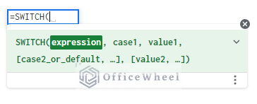
The SWITCH function syntax:
SWITCH(expression, case1, value1, [case2, value2, ...], [default])It is slightly different from MATCH as we can directly determine the priority of each text condition:
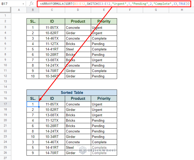
SWITCH(E3:E12,"Urgent",1,"Pending",2,"Complete",3)Now, adding this to the SORT function we get the formula:
=ARRAYFORMULA(SORT(B3:E12,SWITCH(E3:E12,"Urgent",1,"Pending",2,"Complete",3),TRUE))The SWITCH function may be preferable over MATCH as it is simpler to understand.
Read More: How to Sum Using ARRAYFORMULA in Google Sheets
Final Words
That should cover all the ways in which we can apply a custom sort on Google Sheets. Hope that all the methods we have discussed today come in handy in your spreadsheets’ tasks.
Feel free to leave any queries or advice you might have for us in the comments section below.
Related Articles for Reading
- Sort By Column in Google Sheets (3 Easy Ways)
- SORT Function for Multiple Columns in Google Sheets
- How to Sort by Value in Google Sheets (With Examples)
- How to Sort by Number in Google Sheets (4 Ways)
- Sort by Row in Google Sheets (2 Basic Ways)
- How to VLOOKUP Last Match in Google Sheets (5 Simple Ways)
- How to Use Formula to Highlight Duplicates in Google Sheets
- Google Sheets: Convert Text to Number (6 Easy Ways)

